Page 280 - Applied Numerical Methods Using MATLAB

PREDICTOR–CORRECTOR METHOD 269
1

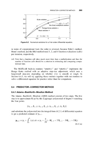
0.8 Euler solution +

0.6 + y(t) = 1 – e –at
the (true) analytical solution
0.4 + Runge-Kutta solution
Heun solution +
0.2
h = 0.5
0
0 0.5 1 1.5 t 2
Figure 6.2 Numerical solutions for a first-order differential equation.

in terms of computational load, the order is reversed, because Euler’s method,
Heun’s method, and the RK4 method need 1, 2, and 4 function evaluations (calls)
per iteration, respectively.

(cf) Note that a function call takes much more time than a multiplication and thus the
number of function calls should be a criterion in estimating and comparing compu-
tational time.

The MATLAB built-in routines “ode23()”and “ode45()” implement the
Runge–Kutta method with an adaptive step-size adjustment, which uses a
large/small step-size depending on whether f(t) is smooth or rough. In
Section 6.4.3, we will try applying these routines together with our routines to
solve a differential equation for practice rather than for comparison.

6.4 PREDICTOR–CORRECTOR METHOD

6.4.1 Adams–Bashforth–Moulton Method
The Adams–Bashforth–Moulton (ABM) method consists of two steps. The first
step is to approximate f(t,y) by the (Lagrange) polynomial of degree 4 matching
the four points

{(t k−3 , f k−3 ), (t k−2 , f k−2 ), (t k−1 , f k−1 ), (t k , f k )}

and substitute the polynomial into the integral form (6.2.1) of differential equation
to get a predicted estimate of y k+1 .

h
h
p k+1 = y k + l 3 (t) dt = y k + (−9f k−3 + 37f k−2 − 59f k−1 + 55f k )
0 24
(6.4.1a)