Page 279 - Applied Numerical Methods Using MATLAB

268 ORDINARY DIFFERENTIAL EQUATIONS

function [t,y] = ode_RK4(f,tspan,y0,N,varargin)
%Runge-Kutta method to solve vector differential eqn y’(t) = f(t,y(t))
% for tspan = [t0,tf] and with the initial value y0 and N time steps
if nargin < 4 | N <= 0, N = 100; end
if nargin < 3, y0 = 0; end
y(1,:) = y0(:)’; %make it a row vector
h = (tspan(2) - tspan(1))/N; t = tspan(1)+[0:N]’*h;
for k = 1:N
f1 = h*feval(f,t(k),y(k,:),varargin{:}); f1 = f1(:)’; %(6.3.2a)
f2 = h*feval(f,t(k) + h/2,y(k,:) + f1/2,varargin{:}); f2 = f2(:)’;%(6.3.2b)
f3 = h*feval(f,t(k) + h/2,y(k,:) + f2/2,varargin{:}); f3 = f3(:)’;%(6.3.2c)
f4 = h*feval(f,t(k) + h,y(k,:) + f3,varargin{:}); f4 = f4(:)’; %(6.3.2d)
y(k + 1,:) = y(k,:) + (f1 + 2*(f2 + f3) + f4)/6; %Eq.(6.3.1)
end
%nm630: Heun/Euer/RK4 method to solve a differential equation (d.e.)
clear, clf
tspan = [0 2];
t = tspan(1)+[0:100]*(tspan(2) - tspan(1))/100;
a=1;yt=1- exp(-a*t); %Eq.(6.1.5): true analytical solution
plot(t,yt,’k’), hold on
df61 = inline(’-y + 1’,’t’,’y’); %Eq.(6.1.1): d.e. to be solved
y0=0; N=4;
[t1,ye] = oed_Euler(df61,tspan,y0,N);
[t1,yh] = ode_Heun(df61,tspan,y0,N);
[t1,yr] = ode_RK4(df61,tspan,y0,N);
plot(t,yt,’k’, t1,ye,’b:’, t1,yh,’b:’, t1,yr,’r:’)
plot(t1,ye,’bo’, t1,yh,’b+’, t1,yr,’r*’)
N = 1e3; %to estimate the time for N iterations
tic, [t1,ye] = ode_Euler(df61,tspan,y0,N); time_Euler = toc
tic, [t1,yh] = ode_Heun(df61,tspan,y0,N); time_Heun = toc
tic, [t1,yr] = ode_RK4(df61,tspan,y0,N); time_RK4 = toc

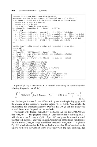
Equation (6.3.1) is the core of RK4 method, which may be obtained by sub-
stituting Simpson’s rule (5.5.4)

t k+1 h x k+1 − x k h
∼
f(x) dx = (f k + 4f k+1/2 + f k+1 ) with h = =
3 2 2
t k
(6.3.3)
into the integral form (6.2.1) of differential equation and replacing f k+1/2 with
the average of the successive function values (f k2 + f k3 )/2. Accordingly, the
4
RK4 method has a truncation error of O(h ) as Eq. (5.6.2) and thus is expected
to work better than the previous two methods.
The fourth-order Runge–Kutta (RK4) method is cast into the MATLAB rou-
tine “ode_RK4()”. The program “nm630.m” uses this routine to solve Eq. (6.1.1)
with the step size h = (t f − t 0 )/N = 2/4 = 0.5 and plots the numerical result
together with the (true) analytical solution. Comparison of this result with those of
Euler’s method (“ode_Euler()”) and Heun’s method (“ode_Heun()”) is given in
Fig. 6.2, which shows that the RK4 method is better than Heun’s method, while
Euler’s method is the worst in terms of accuracy with the same step-size. But,