Page 277 - Applied Numerical Methods Using MATLAB

266 ORDINARY DIFFERENTIAL EQUATIONS
1

0.8
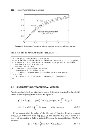
h = 0.25
0.6 h = 0.5

0.4
the (true) analytical solution
y(t) = 1 – e –at
0.2

0
0 0.5 1 1.5 t 2

Figure 6.1 Examples of numerical solution obtained by using the Euler’s method.

and is cast into the MATLAB routine “ode_Euler()”.

function [t,y] = ode_Euler(f,tspan,y0,N)
%Euler’s method to solve vector differential equation y’(t) = f(t,y(t))
% for tspan = [t0,tf] and with the initial value y0 and N time steps
if nargin<4|N<=0, N= 100; end
if nargin<3, y0 = 0; end
h = (tspan(2) - tspan(1))/N; %stepsize
t = tspan(1)+[0:N]’*h; %time vector
y(1,:) = y0(:)’; %always make the initial value a row vector
for k = 1:N
y(k + 1,:) = y(k,:) +h*feval(f,t(k),y(k,:)); %Eq.(6.1.7)
end

6.2 HEUN’S METHOD: TRAPEZOIDAL METHOD

Another method of solving a first-order vector differential equation like Eq. (6.1.6)
comes from integrating both sides of the equation.

t k+1

y (t) = f(t, y), y(t)| t k+1 = y(t k+1 ) − y(t k ) = f(t, y)dt
t k
t k
t k+1

y(t k+1 ) = y(t k ) + f(t, y)dt with y(t 0 ) = y 0 (6.2.1)
t k
If we assume that the value of the (derivative) function f(t,y) is constant
as f(t k ,y(t k )) within one time step [t k ,t k+1 ), this becomes Eq. (6.1.7) (with h =
t k+1 − t k ), amounting to Euler’s method. If we use the trapezoidal rule (5.5.3), it
becomes
h
y k+1 = y k + {f(t k , y k ) + f(t k+1 , y k+1 )} (6.2.2)
2