Page 281 - Applied Numerical Methods Using MATLAB

270 ORDINARY DIFFERENTIAL EQUATIONS
The second step is to repeat the same work with the updated four points

{(t k−2 , f k−2 ), (t k−1 , f k−1 ), (t k , f k ), (t k+1 , f k+1 )} (f k+1 = f(t k+1 , p k+1 ))

to get a corrected estimate of y k+1 .

h h

c k+1 = y k + l (t) dt = y k + (f k−2 − 5f k−1 + 19f k + 9f k+1 ) (6.4.1b)
3
0 24
The coefficients of Eqs. (6.4.1a) and (6.4.1b) can be obtained by using the
MATLAB routines “lagranp()”and “polyint()”, each of which generates
Lagrange (coefficient) polynomials and integrates a polynomial, respectively.
Let’s try running the program “ABMc.m”.

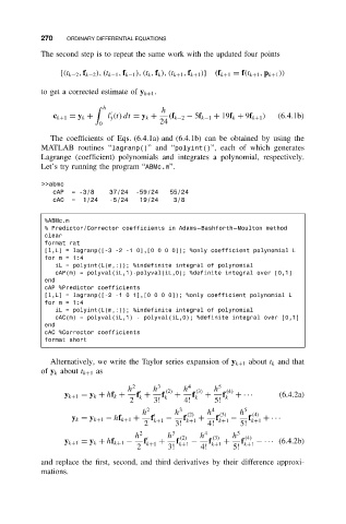
>>abmc
cAP = -3/8 37/24 -59/24 55/24
cAC = 1/24 -5/24 19/24 3/8

%ABMc.m
% Predictor/Corrector coefficients in Adams–Bashforth–Moulton method
clear
format rat
[l,L] = lagranp([-3 -2 -1 0],[0 0 0 0]); %only coefficient polynomial L
for m = 1:4
iL = polyint(L(m,:)); %indefinite integral of polynomial
cAP(m) = polyval(iL,1)-polyval(iL,0); %definite integral over [0,1]
end
cAP %Predictor coefficients
[l,L] = lagranp([-2 -1 0 1],[0 0 0 0]); %only coefficient polynomial L
for m = 1:4
iL = polyint(L(m,:)); %indefinite integral of polynomial
cAC(m) = polyval(iL,1) - polyval(iL,0); %definite integral over [0,1]
end
cAC %Corrector coefficients
format short

Alternatively, we write the Taylor series expansion of y k+1 about t k and that
of y k about t k+1 as

h 2 h 3 h 4 h 5
(2) (3) (4)
y k+1 = y k + hf k + f + f k + f k + f k +· · · (6.4.2a)
k
2 3! 4! 5!
h 2 h 3 (2) h 4 (3) h 5 (4)
y k = y k+1 − hf k+1 + f k+1 − f k+1 + f k+1 − f k+1 +· · ·
2 3! 4! 5!
h 2 h 3 (2) h 4 (3) h 5 (4)
y k+1 = y k + hf k+1 − f k+1 + f k+1 − f k+1 + f k+1 −· · · (6.4.2b)
2 3! 4! 5!
and replace the first, second, and third derivatives by their difference approxi-
mations.