Page 286 - Applied Numerical Methods Using MATLAB

PREDICTOR–CORRECTOR METHOD 275

× 10 −5
1 6
4
0.5
true analytical solution y(t) = 1 − e −t 2
and numerical solutions
0 0
0 2 4 6 8 10 0 2 4 6 8 10
(a1) Numerical solutions without modifiers (b1) Relative errors without modifiers
× 10 −5
1 1.5
RK4
1 ABM
0.5 Hamming
true analytical solution y(t) = 1 − e −t 0.5
and numerical solutions
0 0
0 2 4 6 8 10 0 2 4 6 8 10
(a2) Numerical solutions with modifiers (b2) Relative errors with modifiers

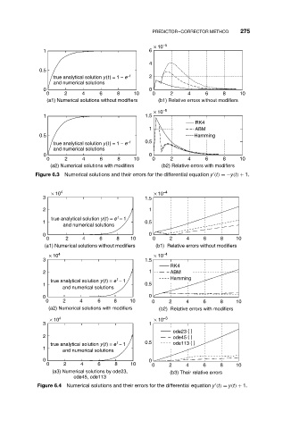
Figure 6.3 Numerical solutions and their errors for the differential equation y (t) =−y(t) + 1.
× 10 4 × 10 –4
3 1.5
2 1
t
true analytical solution y(t) = e − 1
1 0.5
and numerical solutions
0 0
0 2 4 6 8 10 0 2 4 6 8 10
(a1) Numerical solutions without modifiers (b1) Relative errors without modifiers
× 10 4 × 10 –4
3 1.5
RK4
2 1 ABM
t
true analytical solution y(t) = e − 1 Hamming
1 0.5
and numerical solutions
0 0
0 2 4 6 8 10 0 2 4 6 8 10
(a2) Numerical solutions with modifiers (b2) Relative errors with modifiers
× 10 4 × 10 –3
3 1
ode23 ( )
2 ode45 ( )
t
true analytical solution y(t) = e − 1 0.5 ode113 ( )
1
and numerical solutions
0 0
0 2 4 6 8 10 0 2 4 6 8 10
(a3) Numerical solutions by ode23, (b3) Their relative errors
ode45, ode113
Figure 6.4 Numerical solutions and their errors for the differential equation y (t) = y(t) + 1.