Page 289 - Applied Numerical Methods Using MATLAB

278 ORDINARY DIFFERENTIAL EQUATIONS

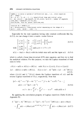
%nm651_1 to solve a system of differential eqs., i.e., state equation
df = ’df651’;
t0 = 0; tf = 2; x0 = [1 -1]; %start/final time and initial value
N = 45; [tH,xH] = ode_Ham(df,[t0 tf],x0,N); %with N = number of segments
[t45,x45] = ode45(df,[t0 tf],x0);
plot(tH,xH), hold on, pause, plot(t45,x45)

function dx = df651(t,x)
dx = zeros(size(x)); %row/column vector depending on the shape of x
dx(1) = x(2); dx(2) = -x(2) + 1;

Especially for the state equations having only constant coefficients like Eq.
(6.5.2), we can change it into a matrix–vector form as

x 1 (t) 0 1 x 1 (t) 0
= + u s (t) (6.5.3)
x 2 (t) 0 −1 x 2 (t) 1

x 1 (0) 1
with = and u s (t) = 1 ∀ t ≥ 0
x 2 (0) −1

x (t) = Ax(t) + Bu(t) with the initial state x(0) and the input u(t) (6.5.4)
which is called a linear time-invariant (LTI) state equation, and then try to find
the analytical solution. For this purpose, we take the Laplace transform of both
sides to write

sX(s) − x(0) = AX(s) + BU(s) with X(s) = L{x(t)},U(s) = L{u(t)}
−1
−1
[sI − A]X(s) = x(0) + BU(s), X(s) = [sI − A] x(0) + [sI − A] BU(s)
(6.5.5)
−1
where L{x(t)} and L {X(s)} denote the Laplace transform of x(t) and the
inverse Laplace transform of X(s), respectively. Note that
2 −2
[sI − A] −1 = s −1 [I − As −1 −1 = s −1 I + As −1 + A s +· · ·
]
−1 −1
φ(t) = L {[sI − A] } (6.5.6)
A 2 2 A 3 3 At
= I + At + t + t +· · · = e with φ(0) = I
2 3!
By applying the convolution property of Laplace transform (Table D.2(4) in
Appendix D)
−1
−1
−1
−1
−1
L {[sI − A] BU(s)}= L {[sI − A] }∗ L {BU(s)}= φ(t) ∗ Bu(t)
∞
t
u(τ)=0for τ<0or τ>t
= φ(t − τ)Bu(τ) dτ = φ(t − τ)Bu(τ) dτ (6.5.7)
−∞ 0