Page 288 - Applied Numerical Methods Using MATLAB

VECTOR DIFFERENTIAL EQUATIONS 277
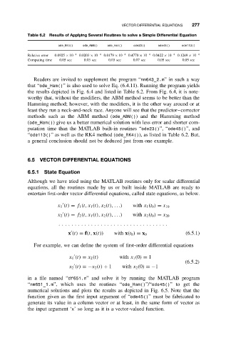
Table 6.2 Results of Applying Several Routines to solve a Simple Differential Equation

ode RK4() ode ABM() ode Ham() ode23() ode45() ode113()
Relative error 0.0925 × 10 −4 0.0203 × 10 −4 0.0179 × 10 −4 0.4770 × 10 −4 0.0422 × 10 −4 0.1249 × 10 −4
Computing time 0.05 sec 0.03 sec 0.03 sec 0.07 sec 0.05 sec 0.05 sec

Readers are invited to supplement the program “nm643_2.m”insuchaway
that “ode_Ham()” is also used to solve Eq. (6.4.11). Running the program yields
the results depicted in Fig. 6.4 and listed in Table 6.2. From Fig. 6.4, it is note-
worthy that, without the modifiers, the ABM method seems to be better than the
Hamming method; however, with the modifiers, it is the other way around or at
least they run a neck-and-neck race. Anyone will see that the predictor–corrector
methods such as the ABM method (ode_ABM()) and the Hamming method
(ode_Ham()) give us a better numerical solution with less error and shorter com-
putation time than the MATLAB built-in routines “ode23()”, “ode45()”, and
“ode113()” as well as the RK4 method (ode_RK4()), as listed in Table 6.2. But,
a general conclusion should not be deduced just from one example.

6.5 VECTOR DIFFERENTIAL EQUATIONS

6.5.1 State Equation

Although we have tried using the MATLAB routines only for scalar differential
equations, all the routines made by us or built inside MATLAB are ready to
entertain first-order vector differential equations, called state equations, as below.

x 1 (t) = f 1 (t, x 1 (t), x 2 (t), . . .) with x 1 (t 0 ) = x 10

x 2 (t) = f 2 (t, x 1 (t), x 2 (t), . . .) with x 2 (t 0 ) = x 20
.. ... .. .. ... .. ... .. .. ... .. .. ... .. .

x (t) = f(t, x(t)) with x(t 0 ) = x 0 (6.5.1)
For example, we can define the system of first-order differential equations

x 1 (t) = x 2 (t) with x 1 (0) = 1
(6.5.2)
x 2 (t) =−x 2 (t) + 1 with x 2 (0) =−1

in a file named “df651.m” and solve it by running the MATLAB program
“nm651_1.m”, which uses the routines “ode_Ham()”/“ode45()”to get the
numerical solutions and plots the results as depicted in Fig. 6.5. Note that the
function given as the first input argument of “ode45()” must be fabricated to
generate its value in a column vector or at least, in the same form of vector as
the input argument ‘x’ so long as it is a vector-valued function.