Page 276 - Applied Numerical Methods Using MATLAB

EULER’S METHOD 265

%nm610: Euler method to solve a 1st-order differential equation
clear, clf
a=1;r=1;y0=0; tf = 2;
t = [0:0.01:tf]; yt=1- exp(-a*t); %Eq.(6.1.5): true analytical solution
plot(t,yt,’k’), hold on
klasts = [8 4 2]; hs = tf./klasts;
y(1) = y0;
for itr = 1:3 %with various step size h = 1/8,1/4,1/2
klast = klasts(itr); h = hs(itr); y(1)=y0;
for k = 1:klast
y(k + 1) = (1 - a*h)*y(k) +h*r; %Eq.(6.1.3):
plot([k - 1 k]*h,[y(k) y(k+1)],’b’, k*h,y(k+1),’ro’)
ifk<4, pause; end
end
end

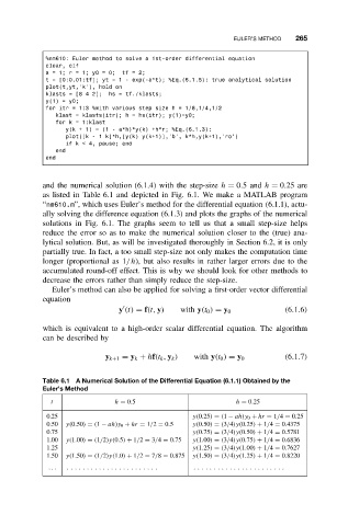
and the numerical solution (6.1.4) with the step-size h = 0.5and h = 0.25 are
as listed in Table 6.1 and depicted in Fig. 6.1. We make a MATLAB program
“nm610.m”, which uses Euler’s method for the differential equation (6.1.1), actu-
ally solving the difference equation (6.1.3) and plots the graphs of the numerical
solutions in Fig. 6.1. The graphs seem to tell us that a small step-size helps
reduce the error so as to make the numerical solution closer to the (true) ana-
lytical solution. But, as will be investigated thoroughly in Section 6.2, it is only
partially true. In fact, a too small step-size not only makes the computation time
longer (proportional as 1/h), but also results in rather larger errors due to the
accumulated round-off effect. This is why we should look for other methods to
decrease the errors rather than simply reduce the step-size.
Euler’s method can also be applied for solving a first-order vector differential
equation
y (t) = f(t, y) with y(t 0 ) = y 0 (6.1.6)

which is equivalent to a high-order scalar differential equation. The algorithm
can be described by

y k+1 = y k + hf(t k , y k ) with y(t 0 ) = y 0 (6.1.7)

Table 6.1 A Numerical Solution of the Differential Equation (6.1.1) Obtained by the
Euler’s Method
t h = 0.5 h = 0.25

0.25 y(0.25) = (1 − ah)y 0 + hr = 1/4 = 0.25
0.50 y(0.50) = (1 − ah)y 0 + hr = 1/2 = 0.5 y(0.50) = (3/4)y(0.25) + 1/4 = 0.4375
0.75 y(0.75) = (3/4)y(0.50) + 1/4 = 0.5781
1.00 y(1.00) = (1/2)y(0.5) + 1/2 = 3/4 = 0.75 y(1.00) = (3/4)y(0.75) + 1/4 = 0.6836
1.25 y(1.25) = (3/4)y(1.00) + 1/4 = 0.7627
1.50 y(1.50) = (1/2)y(1.0) + 1/2 = 7/8 = 0.875 y(1.50) = (3/4)y(1.25) + 1/4 = 0.8220
... .... ....... ....... ..... ..... ....... ....... ....