Page 385 - Applied Numerical Methods Using MATLAB

374 MATRICES AND EIGENVALUES
Then, noting that the modal matrix V is nonsingular and invertible by Theo-
rem 8.1, we can premultiply the above equation by the inverse modal matrix
V −1 to get
−1 −1
V AV = V V ≡ (8.2.4)

This implies that the modal matrix composed of the eigenvectors of a matrix A
is the similarity transformation matrix that can be used for converting the matrix
A into a diagonal matrix having its eigenvalues on the main diagonal. Here is an
example to illustrate the diagonalization.

Example 8.2. Diagonalization Using the Modal Matrix.
Consider the matrix given in the previous example.

0 1
A = (E8.2.1)
0 −1
We can use the eigenvectors (E8.1.3) (obtained in Example 8.1) to construct
the modal matrix as
√
1 1/ 2
V = [v 1 v 2 ] = √ (E8.2.2)
0 −1/ 2
and use this matrix to make a similarity transformation of the matrix A as

√
1 1/ 2 0 1 1 1/ 2
√ −1
V −1 AV = √ √
0 −1/ 2 0 −1 0 −1/ 2
√
1 1 0 −1/ 2 0 0
= √ √ = (E8.2.3)
0 − 2 0 1/ 2 0 −1
which is a diagonal matrix having the eigenvalues on its main diagonal.
This job can be performed by the last statement of the MATLAB program
“nm811.m”.

This diagonalization technique can be used to decouple an N-dimensional
vector differential equation so that it can be as easy to solve as N independent
scalar differential equations. Here is an illustration.

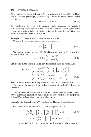
Example 8.3. Decoupling of a Vector Equation Through Diagonalization
(a) For the linear time-invariant (LTI) state equation (6.5.3)

x 1 (t) 0 1 x 1 (t) 0
= + u s (t) (E8.3.1)

x 2 (t) 0 −1 x 2 (t) 1

x 1 (0) 1
with = and u s (t) = 1 ∀ t ≥ 0
x 2 (0) −1

x (t) = Ax(t) + Bu(t) with the initial state x(0) and the input u(t)