Page 387 - Applied Numerical Methods Using MATLAB

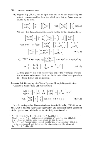
376 MATRICES AND EIGENVALUES
(b) Suppose Eq. (E8.3.1) has no input term and so we can expect only the
natural response resulting from the initial state, but no forced response
caused by the input.

x 1 (t) 0 1 x 1 (t) x 1 (0) 1
= with = (E8.3.7)
x 2 (t) 0 −1 x 2 (t) x 2 (0) 1

We apply the diagonalization/decoupling method for this equation to get

w 1 (t) λ 1 0 w 1 (t) 0 0 w 1 (t)

= =

w 2 (t) 0 λ 2 w 2 (t) 0 −1 w 2 (t)

w 1 (0) 1 1 1 2
−1
with w(0) = V x(0), = √ = √
w 2 (0) 0 − 2 1 − 2
λ 1 t
w 1 (t) w 1 (0)e 2
= λ 2 t = √ (E8.3.8)
w 2 (t) w 2 (0)e − 2e −t
λ 1 t
(E8.3.2) w 1 (0)e λ 1 t λ 2 t
x(t) = V w(t) = [v 1 v 2 ] λ 2 t = w 1 (0)e v 1 + w 2 (0)e v 2
w 2 (0)e
√ −t
1 1/ 2 2 2 − e
= √ √ −t = −t (E8.3.9)
0 −1/ 2 − 2e e
As time goes by, this solution converges and so the continuous-time sys-
tem turns out to be stable, thanks to the fact that all of the eigenvalues
(0, −1) are distinct and not positive.
Example 8.4. Decoupling of a Vector Equation Through Diagonalization.
Consider a discrete-time LTI state equation

x 1 [n + 1] 0 1 x 1 [n] 0
= + u s [n]
x 2 [n + 1] 0.20.1 x 2 [n] 2.2361

x 1 [0] 1
with = and u s [n] = 1 ∀ n ≥ 0 (E8.4.1)
x 2 [0] −1
In order to diagonalize this equation into a form similar to Eq. (E8.3.4), we use
MATLAB to find the eigenvalues/eigenvectors and the modal matrix composed
of the eigenvectors and finally, do the similarity transformation.

A = [0 1;0.2 0.1]; B = [0; 2.2361]; % Eq.(E8.4.1)
[V,L] = eig(A)%V= modal matrix composed of eigenvectors (E8.4.2)
% L = diagonal matrix with eigenvalues on its diagonal
Ap = V^-1*A*V %diagonalize through similarity transformation (E8.4.3)
% into a diagonal matrix having the eigenvalues on the diagonal
Bp = V^-1*B % (E8.4.3)