Page 388 - Applied Numerical Methods Using MATLAB

SIMILARITY TRANSFORMATION AND DIAGONALIZATION 377
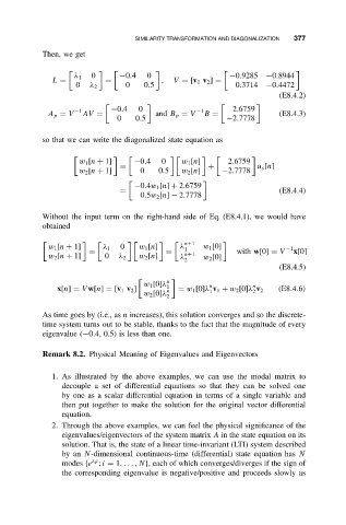
Then, we get

0 −0.4 0 −0.9285 −0.8944
λ 1
L = = , V = [v 1 v 2 ] =
0 λ 2 0 0.5 0.3714 −0.4472
(E8.4.2)

−0.4 0 −1 2.6759
−1
A p = V AV = and B p = V B = (E8.4.3)
0 0.5 −2.7778
so that we can write the diagonalized state equation as

w 1 [n + 1] −0.4 0 w 1 [n] 2.6759
= + u s [n]
w 2 [n + 1] 0 0.5 w 2 [n] −2.7778

−0.4w 1 [n] + 2.6759
= (E8.4.4)
0.5w 2 [n] − 2.7778
Without the input term on the right-hand side of Eq. (E8.4.1), we would have
obtained

n+1
w 1 [n + 1] λ 1 0 w 1 [n] λ 1 w 1 [0] −1
= = with w[0] = V x[0]
w 2 [n + 1] 0 λ 2 w 2 [n] λ n+1 w 2 [0]
2
(E8.4.5)
n
w 1 [0]λ n n
x[n] = V w[n] = [v 1 v 2 ] 1 n = w 1 [0]λ v 1 + w 2 [0]λ v 2 (E8.4.6)
2
1
w 2 [0]λ
2
As time goes by (i.e., as n increases), this solution converges and so the discrete-
time system turns out to be stable, thanks to the fact that the magnitude of every
eigenvalue (−0.4, 0.5) is less than one.

Remark 8.2. Physical Meaning of Eigenvalues and Eigenvectors

1. As illustrated by the above examples, we can use the modal matrix to
decouple a set of differential equations so that they can be solved one
by one as a scalar differential equation in terms of a single variable and
then put together to make the solution for the original vector differential
equation.
2. Through the above examples, we can feel the physical significance of the
eigenvalues/eigenvectors of the system matrix A in the state equation on its
solution. That is, the state of a linear time-invariant (LTI) system described
by an N-dimensional continuous-time (differential) state equation has N
λ i t
modes {e ; i = 1,...,N}, each of which converges/diverges if the sign of
the corresponding eigenvalue is negative/positive and proceeds slowly as