Page 393 - Applied Numerical Methods Using MATLAB

382 MATRICES AND EIGENVALUES
Theorem 8.3. Symmetric Diagonalization Theorem.
All of the eigenvalues of an N × N symmetric matrix A are of real value and
its eigenvectors form an orthonormal basis of an N-dimensional linear space.
Consequently, we can make an orthonormal modal matrix V composed of the
T
eigenvectors such that V V = I; V −1 = V T and use the modal matrix to make
the similarity transformation of A, which yields a diagonal matrix having the
eigenvalues on its main diagonal:

T
V AV = V −1 AV = (8.4.1)

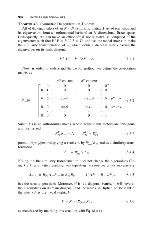
Now, in order to understand the Jacobi method, we define the pq-rotation
matrix as

th
th
p column q column
1 0 · 0 · 0 · 0
 
 0 1 · 0 · 0 · 0 
 
 · · · · · · · · 
th
 0 0 · cos θ · − sin θ · 0  p row


(8.4.2)
 · · · · · · · · 

R pq (θ) = 
th
 0 0 · sin θ · cos θ · 0  q row


· · · · · · · ·
 
0 0 · 0 · 0 · 1
Since this is an orthonormal matrix whose row/column vectors are orthogonal
and normalized
T
R R pq = I, R T = R −1 (8.4.3)
pq pq pq
T
premultiplying/postmultiplying a matrix A by R /R pq makes a similarity trans-
pq
formation
T
A (1) = R AR pq (8.4.4)
pq
Noting that the similarity transformation does not change the eigenvalues (Re-
mark 8.1), any matrix resulting from repeating the same operations successively
T
T
A (k+1) = R A (k) R (k) = R R T T (8.4.5)
(k) (k) (k−1) ··· R AR ··· R (k−1) R (k)
has the same eigenvalues. Moreover, if it is a diagonal matrix, it will have all
the eigenvalues on its main diagonal, and the matrix multiplied on the right of
the matrix A is the modal matrix V
V = R ··· R (k−1) R (k) (8.4.6)
as manifested by matching this equation with Eq. (8.4.1).