Page 397 - Applied Numerical Methods Using MATLAB

386 MATRICES AND EIGENVALUES
can be written as
N
λ n t
x(t) = e α n v n (8.5.8)
n=1
Equations (8.5.6) and (8.5.8) imply that the eigenvalues of the system matrix
characterize the principal modes of the system described by the state equations.
That is, the eigenvalues determine not only whether the system is stable or
not—that is, whether the system state converges to an equilibrium state or
diverges—but also how fast the system state proceeds along the direction of
each eigenvector. More specifically, in the case of a discrete-time system, the
absolute values of all the eigenvalues must be less than one for stability and
the smaller the absolute value of an eigenvalue (less than one) is, the faster the
corresponding mode converges. In the case of a continuous-time system, the real
parts of all the eigenvalues must be negative for stability and the smaller a neg-
ative eigenvalue is, the faster the corresponding mode converges. The difference
among the eigenvalues determines how stiff the system is (see Section 6.5.4).
This meaning of eigenvalues/eigenvectors is very important in dynamic systems.
Now, in order to figure out the meaning of eigenvalues/eigenvectors in static
systems, we define the mean vector and the covariance matrix of the vectors
(1)
(2)
{x , x ,..., x (K) } representing K points in a two-dimensional space called the
x 1 x 2 plane as
K K
1 (k) 1 (k) (k) T
m x = x , C x = [x − m x ][x − m x ] (8.5.9)
K K
k=1 k=1
where the mean vector represents the center of the points and the covariance
matrix describes how dispersedly the points are distributed. Let us think about
the geometrical meaning of diagonalizing the covariance matrix C x .Asa simple
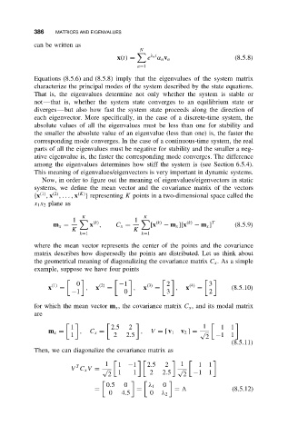
example, suppose we have four points

0 (2) −1 (3) 2 (4) 3
(1)
x = , x = , x = , x = (8.5.10)
−1 0 3 2
for which the mean vector m x , the covariance matrix C x , and its modal matrix
are

1 2.5 2 1 11
m x = , C x = , V = [ v 1 v 2 ] = √
1 2 2.5 2 −11
(8.5.11)
Then, we can diagonalize the covariance matrix as
1 1 −1 2.5 2 1 1 1
T
V C x V = √ √
2 1 1 2 2.5 2 −11

0.5 0 λ 1 0
= = = (8.5.12)
0 4.5 0 λ 2