Page 401 - Applied Numerical Methods Using MATLAB

390 MATRICES AND EIGENVALUES
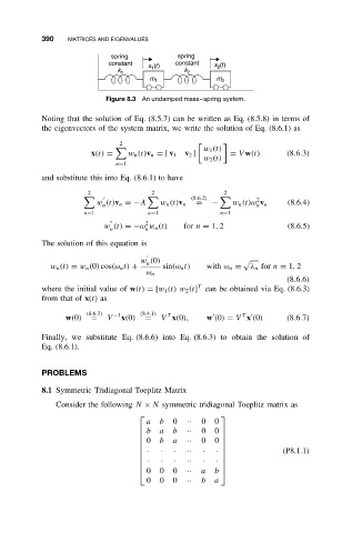
spring spring
constant x 1 (t) constant x 2 (t)
k 1 k 2
m 1 m 2

Figure 8.3 An undamped mass–spring system.

Noting that the solution of Eq. (8.5.7) can be written as Eq. (8.5.8) in terms of
the eigenvectors of the system matrix, we write the solution of Eq. (8.6.1) as
2
w 1 (t)
x(t) = w n (t)v n = [ v 1 v 2 ] = V w(t) (8.6.3)
w 2 (t)
n=1
and substitute this into Eq. (8.6.1) to have

2 2 2
(8.6.2)
2
w (t)v n =−A = − (8.6.4)
n w n (t)v n w n (t)ω v n
n
n=1 n=1 n=1
2
w (t) =−ω w n (t) for n = 1, 2 (8.6.5)
n
n
The solution of this equation is

w (0)
n
w n (t) = w n (0) cos(ω n t) + sin(ω n t) with ω n = λ n for n = 1, 2
ω n
(8.6.6)
T
where the initial value of w(t) = [w 1 (t) w 2 (t] can be obtained via Eq. (8.6.3)
from that of x(t)as
(8.6.3) −1 (8.4.1) T
T

w(0) = V x(0) = V x(0), w (0) = V x (0) (8.6.7)
Finally, we substitute Eq. (8.6.6) into Eq. (8.6.3) to obtain the solution of
Eq. (8.6.1).
PROBLEMS
8.1 Symmetric Tridiagonal Toeplitz Matrix

Consider the following N × N symmetric tridiagonal Toeplitz matrix as
 
a b 0 ·· 0 0
 b a b ·· 0 0 

 0 b a ·· 0 0 

 
· · · ·· · · (P8.1.1)
 
 
· · · ·· · ·
 
 
0 0 0 ·· a b
 
0 0 0 ·· b a