Page 400 - Applied Numerical Methods Using MATLAB

EIGENVALUE EQUATIONS 389

x 2 (2) x 2
x = (x 12 , x 22 )
x 22
y (2)

R(−q 1 )
q 2 x 11
x 1
q 1 < 0 x 12
q 2 − q 1 (1)
y
x 1
2 2
x 21 (1) x 11 + x 21
x = (x 11 , x 21 )
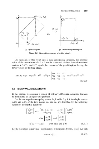
(a) A parallelogram (b) The rotated parallelogram
Figure 8.2 Geometrical meaning of a determinant.

On extension of this result into a three-dimensional situation, the absolute
value of the determinant of a 3 × 3 matrix composed of three three-dimensional
(2)
(1)
vectors x , x ,and x (3) equals the volume of the parallelepiped having the
three vectors as its three edges.

x

11 x 12 x 13
det(X) =|X|=| x (1) x (2) x (3) |= x 21 x 22 x 23 ≡ x (1) × x (2) · x (3)

x 31 x 32 x 33

(8.5.22)
8.6 EIGENVALUE EQUATIONS
In this section, we consider a system of ordinary differential equations that can
be formulated as an eigenvalue problem.
For the undamped mass–spring system depicted in Fig. 8.3, the displacements
x 1 (t) and x 2 (t) of the two masses m 1 and m 2 are described by the following
system of differential equations:

x (t) x 1 (t)
1 =− (k 1 + k 2 )/m 1 −k 2 /m 1

x (t) −k 2 /m 2 k 2 /m 2 x 2 (t)
2

x 1 (0) x (0)
with and 1
x 2 (0) x (0)

2

x (t) =−Ax(t) with x(0) and x (0) (8.6.1)
2
Let the eigenpairs (eigenvalue–eigenvectors) of the matrix A be (λ n = ω , v n ) with
n
2
Av n = ω v n (8.6.2)
n