Page 395 - Applied Numerical Methods Using MATLAB

384 MATRICES AND EIGENVALUES
th
v pn = v np = a pn c + a qn s for the p row/column with n = p, q (8.4.7b)
th
v qn = v np =−a pn s + a qn c for the q row/column with n = p, q (8.4.7c)
2
2
2
2
v pp = a pp c + a qq s + 2a pq sc = a pp c + a qq s + a pq sin 2θ (8.4.7d)
2
2
2
2
v qq = a pp s + a qq c − 2a pq sc = a pp s + a qq c − a pq sin 2θ (8.4.7e)
(c = cos θ, s = sin θ)
we make the (p, q) element v pq and the (q, p) element v qp zero
v pq = v qp = 0 (8.4.8)
by choosing the angle θ of the rotation matrix R pq (θ) in such a way that

sin 2θ 2a pq 1 1
tan 2θ = = , cos 2θ = = √ ,
2
cos 2θ a pp − a qq sec 2θ 1 + tan 2θ
sin 2θ = tan 2θ cos 2θ (8.4.9)
√
sin 2θ
2
cos θ = cos θ = (1 + cos 2θ)/2, sin θ =
2cos θ
and computing the other associated elements according to Eqs. (8.4.7b–e).
There are a couple of things to note. First, in order to make the matrix closer
to a diagonal one at each iteration, we should identify the row number and the
column number of the largest off-diagonal element as p and q, respectively, and
zero-out the (p, q) element. Second, we can hope that the magnitudes of the
other elements in the pth,qth row/column affected by this transformation process
don’t get larger, since Eqs. (8.4.7b) and (8.4.7c) implies

2
2
v 2 + v 2 = (a pn c + a qn s) + (−a pn s + a qn c) = a 2 + a 2 (8.4.10)
pn qn pn qn
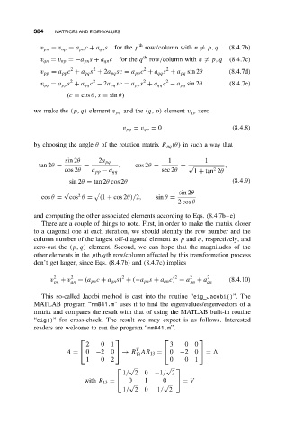
This so-called Jacobi method is cast into the routine “eig_Jacobi()”. The
MATLAB program “nm841.m” uses it to find the eigenvalues/eigenvectors of a
matrix and compares the result with that of using the MATLAB built-in routine
“eig()” for cross-check. The result we may expect is as follows. Interested
readers are welcome to run the program “nm841.m”.

   
2 0 1 3 0 0
T
A =  0 −20  → R AR 13 =  0 −20  =
13
1 0 2 0 0 1
√
 √ 
1/ 20 −1/ 2
with R 13 =  0 1 0  = V
√ √
1/ 20 1/ 2