Page 398 - Applied Numerical Methods Using MATLAB

PHYSICAL MEANING OF EIGENVALUES/EIGENVECTORS 387
which has the eigenvalues on its main diagonal. On the other hand, if we trans-
form the four point vectors by using the modal matrix as

T
y = V (x − m x ) (8.5.13)

then the new four point vectors are

√ √ √ √
1/ 2 −1/ 2 −1/ 2 1/ 2
y (1) = √ , y (2) = √ , y (3) = √ , y (4) = √
−3/ 2 −3/ 2 3/ 2 3/ 2
(8.5.14)
for which the mean vector m x and the covariance matrix C x are

0 0.5 0
T T
m y = V (m x − m x ) = , C y = V C x V = =
0 0 4.5
(8.5.15)
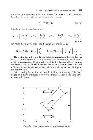
The original four points and the new points corresponding to them are depicted
in Fig. 8.1, which shows that the eigenvectors of the covariance matrix for a set of
point vectors represents the principal axes of the distribution and its eigenvalues
are related with the lengths of the distribution along the principal axes. The
difference among the eigenvalues determines how oblong the overall shape of
the distribution is.
Before closing this section, we may think about the meaning of the deter-
minant of a matrix composed of two two-dimensional vectors and three three-
dimensional vectors.

x (3)
3
x 2
y (3) y (4)
2 x (4)

1
v 2
x (2)
0
x 1
v 1
−1 x (1)

−2
y (2) y (1)
−3
−4 −2 0 2 4

Figure 8.1 Eigenvalues/eigenvectors of a covariance matrix.