Page 126 - Applied Probability

6. Applications of Identity Coefficients
110
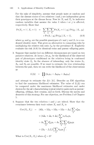
For the sake of simplicity, assume that people mate at random and
that the disease states of two relatives i and j are independent given
their genotypes at the disease locus. Now let X i and X j be indicator
random variables that assume the value 1 when i or j is affected,
respectively. Show that

Pr(X j =1 | X i =1) = Pr(X j =1 | g j )Pr(g j | S r ,g i )
g i g j S r
× Pr(S r | g i )Pr(g i | X i =1), (6.9)
where g i and g j are the possible genotypes of i and j and S r is a con-
densed identity state. This gives an alternative to computing risks by
multiplying the relative risk ratio λ R by the prevalence K. Explicitly
evaluate the risk (6.9) for identical twins and parent–offspring pairs.
3. Suppose that marker loci on different chromosomes are typed on two
putative relatives. At locus i,let p ij be the likelihood of the observed
pair of phenotypes conditional on the relatives being in condensed
identity state S j . In the absence of inbreeding, only the states S 7 ,
S 8 , and S 9 are possible. If we want to estimate the true relationship
between the pair, then we can write the likelihood of the observations
as

L(∆) = (∆ 7 p i7 +∆ 8 p i8 +∆ 9 p i9 )
i
and attempt to estimate the ∆’s [11]. Describe an EM algorithm
to find the maximum likelihood estimates. The value of L(∆) can
be compared under the maximum likelihood estimates and under
choices for the ∆’s characterizing typical relative pairs such as parent–
offspring, siblings, first cousins, and so forth. Discuss the merits and
demerits of this strategy. For one objection, see Problem 2 of Chapter
5.
4. Suppose that the two relatives i and j are inbred. Show that the
covariance between their trait values X i and X j is
2
Cov(X i ,X j ) = (4∆ 1 +2∆ 3 +2∆ 5 +2∆ 7 +∆ 8 ) α p k
k
k

+ (4∆ 1 +∆ 3 +∆ 5 ) α k δ kk p k
k

2 2
+∆ 1 δ p k +∆ 7 δ p k p l
kl
kk
k k l
2

+(∆ 2 − f i f j ) δ kk p k .
k
2
What is Cov(X i ,X j ) when σ =0?
d