Page 121 - Applied Probability

6. Applications of Identity Coefficients
Again in obvious notation, the joint probability of i and j both being
affected is approximately
=E[(Y i + Z i )(Y j + Z j )]
KK R
=E(Y i Y j )+ E(Y i )E(Z j )+ E(Y j )E(Z i )+ E(Z i Z j ) 105
= K 1 K 1R +2K 1K 2 + K 2 K 2R .
The equations for K and KK R can be combined to yield
KK R − K 2 = K 1 K 1R +2K 1K 2 + K 2 K 2R − (K 1 + K 2 ) 2
2
2
= K (λ 1R − 1) + K (λ 2R − 1), (6.6)
1 2
2
where λ 1R = K 1R /K 1 and λ 2R = K 2R /K 2 . Dividing (6.6) by K now gives
2 2

K 1 K 2
λ R − 1= (λ 1R − 1) + (λ 2R − 1),
K K
with λ R = K R /K.
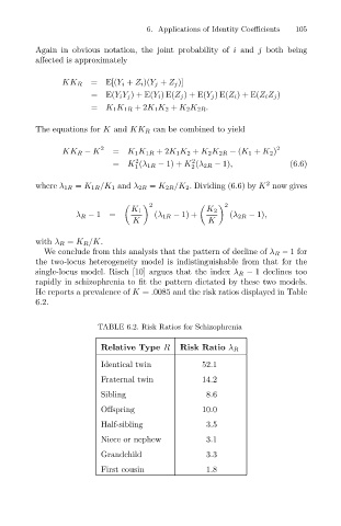
We conclude from this analysis that the pattern of decline of λ R − 1 for
the two-locus heterogeneity model is indistinguishable from that for the
single-locus model. Risch [10] argues that the index λ R − 1 declines too
rapidly in schizophrenia to fit the pattern dictated by these two models.
He reports a prevalence of K = .0085 and the risk ratios displayed in Table
6.2.

TABLE 6.2. Risk Ratios for Schizophrenia

Relative Type R Risk Ratio λ R

Identical twin 52.1
Fraternal twin 14.2
Sibling 8.6
Offspring 10.0

Half-sibling 3.5
Niece or nephew 3.1
Grandchild 3.3
First cousin 1.8