Page 119 - Applied Probability

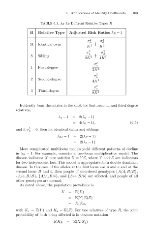
TABLE 6.1. λ R for Different Relative Types R
R
Adjusted Risk Ratios λ R − 1
2
2
σ
σ
a
d
+
Identical twin
M Relative Type 6. Applications of Identity Coefficients 103
2
2
K K
σ 2 a σ 2 d
S Sibling 2 + 2
2K 4K
σ a 2
1 First-degree 2
2K
σ a 2
2 Second-degree 2
4K
σ a 2
3 Third-degree 2
8K
Evidently from the entries in the table for first, second, and third-degree
relatives,
λ 1 − 1= 2(λ 2 − 1)
=4(λ 3 − 1), (6.5)
2
and if σ = 0, then for identical twins and siblings
d
λ M − 1= 2(λ S − 1)
=2(λ 1 − 1).
More complicated multilocus models yield different patterns of decline
in λ R − 1. For example, consider a two-locus multiplicative model. The
disease indicator X now satisfies X = YZ, where Y and Z are indicators
for two independent loci. This model is appropriate for a double-dominant
disease. In this case, if the alleles at the first locus are A and a and at the
second locus B and b, then people of unordered genotypes {A/A, B/B},
{A/a, B/B}, {A/A, B/b}, and {A/a, B/b} are affected, and people of all
other genotypes are normal.
As noted above, the population prevalence is
K =E(X)
=E(Y )E(Z)
= K 1K 2 ,
with K 1 =E(Y ) and K 2 =E(Z). For two relatives of type R, the joint
probability of both being affected is in obvious notation

KK R =E(X i X j )