Page 120 - Applied Probability

6. Applications of Identity Coefficients
104
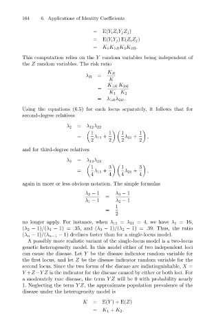
=E(Y i Z i Y j Z j )
=E(Y i Y j )E(Z i Z j )
= K 1 K 1R K 2 K 2R .
This computation relies on the Y random variables being independent of
the Z random variables. The risk ratio
K R
=
λ R
K
K 1R K 2R
=
K 1 K 2
= λ 1R λ 2R .
Using the equations (6.5) for each locus separately, it follows that for
second-degree relatives
λ 2 = λ 12 λ 22
1 1 1 1

= λ 11 + λ 21 + ,
2 2 2 2
and for third-degree relatives
λ 3 = λ 13 λ 23
1 3 1 3

= λ 11 + λ 21 + ,
4 4 4 4
again in more or less obvious notation. The simple formulas

λ 2 − 1 λ 3 − 1
=
λ 1 − 1 λ 2 − 1
1
=
2
no longer apply. For instance, when λ 11 = λ 21 = 4, we have λ 1 = 16,
(λ 2 − 1)/(λ 1 − 1) = .35, and (λ 3 − 1)/(λ 2 − 1) = .39. Thus, the ratio
(λ n − 1)/(λ n−1 − 1) declines faster than for a single-locus model.
A possibly more realistic variant of the single-locus model is a two-locus
genetic heterogeneity model. In this model either of two independent loci
can cause the disease. Let Y be the disease indicator random variable for
the first locus, and let Z be the disease indicator random variable for the
second locus. Since the two forms of the disease are indistinguishable, X =
Y +Z−YZ is the indicator for the disease caused by either or both loci. For
a moderately rare disease, the term YZ will be 0 with probability nearly
1. Neglecting the term YZ, the approximate population prevalence of the
disease under the heterogeneity model is
K =E(Y )+ E(Z)
= K 1 + K 2 .