Page 115 - Applied Probability

6. Applications of Identity Coefficients
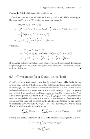
Example 6.2.1 Siblings at the ABO Locus
Consider two non-inbred siblings i and j and their ABO phenotypes.
Because Pr(S r | i = A/B)=∆ r , we have, for example,
Pr(j = A/B | i = A/B) 99
1 1
= Pr(j = A/B | S 7 ,i = A/B)+ Pr(j = A/B | S 8 ,i = A/B)
4 2
1
+ Pr(j = A/B | S 9 ,i = A/B)
4

1 1 1 1 1
= × 1+ p A + p B + 2p Ap B .
4 2 2 2 4
Similarly,
Pr(j = A | i = O/O)
=Pr(j = A/A | i = O/O) + Pr(j = A/O | i = O/O)
1 1 1 2 1 1 1
= × 0+ × 0+ p + × 0+ p A + 2p Ap O .
A
4 2 4 4 2 4
If we assign i either phenotype A or phenotype B, then we must decompose
i’s phenotype into its constituent genotypes. Problem 2 addresses compli-
cations of this sort.

6.3 Covariances for a Quantitative Trait

Consider a quantitative trait controlled by a single locus in Hardy-Weinberg
equilibrium. Let the kth allele a k at the determining locus have population
frequency p k . In the absence of environmental effects, a non-inbred person
with ordered genotype a k /a l has constant trait value µ kl = µ lk . No gener-
ality is lost if we standardize all trait values so that the random value X of

a non-inbred person has mean E(X)= µ kl p k p l = 0. In quantitative
k l
genetics, an additive decomposition µ kl = α k +α l is sought. Because such a
decomposition may not be possible, the allelic contributions α k are chosen
to minimize the deviations δ kl = µ kl − α k − α l . The classical way of doing
this is to minimize the sum of squares
2 2

δ p k p l = (µ kl − α k − α l ) p k p l . (6.1)
kl
k l k l
Setting the partial derivative of (6.1) with respect to α k equal to 0 gives

0= −4 (µ kl − α k − α l )p k p l
l

δ kl p l .
= −4p k
l