Page 285 - Applied Probability

12. Models of Recombination
273
12.7 Application to Drosophila Data
As an application of the various recombination models, we now briefly dis-
cuss the classic Drosophila data of Morgan et al. [20]. These early geneticists
phenotyped 16,136 flies at 9 loci covering almost the entire Drosophila X
chromosome. Because of the nature of the genetic cross employed, a fly
corresponds to a gamete scorable on each interlocus interval as recombi-
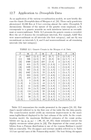
nant or nonrecombinant. Table 12.1 presents the gamete counts n recorded.
Here the set S denotes the recombinant intervals. For example, 6,607 flies
were nonrecombinant on all intervals (the first category), and one fly was
recombinant on intervals 5, 6, and 8 and nonrecombinant on all remaining
intervals (the last category).
TABLE 12.1. Gamete Counts in the Morgan et al. Data
S n S n S n S n
φ 6607 {2, 4} 38 {6, 7} 21 {2, 5, 6} 3
{1} 506 {2, 5} 85 {6, 8} 30 {2, 5, 7} 4
{2} 1049 {2, 6} 237 {7, 8} 2 {2, 5, 8} 1
{3} 855 {2, 7} 123 {1, 2, 3} 1 {2, 6, 7} 2
{4} 1499 {2, 8} 70 {1, 2, 6} 1 {2, 6, 8} 3
{5} 937 {3, 4} 22 {1, 3, 5} 1 {2, 7, 8} 2
{6} 1647 {3, 5} 55 {1, 4, 5} 1 {3, 4, 7} 2
{7} 683 {3, 6} 177 {1, 4, 6} 1 {3, 4, 8} 1
{8} 379 {3, 7} 88 {1, 4, 7} 2 {3, 5, 6} 1
{1, 2} 3 {3, 8} 38 {1, 4, 8} 1 {3, 5, 7} 2
{1, 3} 6 {4, 5} 41 {1, 5, 7} 2 {3, 5, 8} 3
{1, 4} 41 {4, 6} 198 {1, 5, 8} 1 {3, 6, 7} 1
{1, 5} 55 {4, 7} 159 {1, 6, 8} 1 {3, 6, 8} 1
{1, 6} 118 {4, 8} 91 {2, 3, 6} 1 {4, 5, 8} 1
{1, 7} 54 {5, 6} 35 {2, 4, 6} 4 {4, 6, 8} 4
{1, 8} 34 {5, 7} 49 {2, 4, 7} 5 {4, 7, 8} 1
{2, 3} 3 {5, 8} 40 {2, 4, 8} 6 {5, 6, 8} 1

Table 12.2 summarizes the results presented in the papers [18, 23]. Hal-
dane’s model referred to in the first row of the table fits the data poorly.
The count-location model yields an enormous improvement in the maxi-
mum loglikelihood displayed in the last column of the table. In the count-
location model, the maximum likelihood estimates of the count proba-
bilities are (q 0 ,q 1 ,q 2 ,q 3 )=(.06,.41,.48,.05); these estimates correct the
slightly erroneous values given in [23]. The departure of the count proba-
bilities from a Poisson distribution is one of the reasons Haldane’s model
fails so miserably. The chi-square and mixture models referred to in Table
12.2 are special cases of the Poisson-skip model. The best fitting chi-square