Page 336 - Applied Probability

15.5 Process Moments
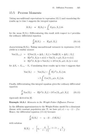
Taking unconditional expectations in expression (15.1) and cumulating the
results up to time t suggests the integral equation
t 15. Diffusion Processes 325
E(X t )=E(X 0 )+ E[µ(s, X s )] ds
0
for the mean E(X t ). Differentiating this result with respect to t provides
the ordinary differential equation
d
E(X t )=E[µ(t, X t )] (15.14)
dt
characterizing E(X t ). Taking unconditional variances in expression (15.2)
yields in a similar manner

Var(X t+s ) = E[Var(X t +∆X t | X t )] + Var[E(X t +∆X t | X t )]
2
=E[σ (t, X t )s + o(s)] + Var[X t + µ(t, X t )s + o(s)]
2
=E[σ (t, X t )]s + Var(X t )+ 2 Cov[X t ,µ(t, X t )]s + o(s)
for ∆X t = X t+s − X t . Cumulating these results up to time t suggests that

t
2
Var(X t )=Var(X 0 )+ E[σ (s, X s )] ds
0
t

+2 Cov[X s ,µ(s, X s )] ds.
0
Finally, differentiating this integral equation gives the ordinary differential
equation
d 2
Var(X t )=E[σ (t, X t )] + 2 Cov[X t ,µ(t, X t )] (15.15)
dt
rigorously derived in [6].

Example 15.5.1 Moments in the Wright-Fisher Diffusion Process
In the diffusion approximation to the Wright-Fisher model for a dominant
disease with constant population size N, we have µ(t, x)= η − (1 − f)x.
Hence, the differential equation (15.14) becomes

d
E(X t ) = η − (1 − f)E(X t )
dt
with solution

η −(1−f)t η
E(X t )= x 0 − e +
1 − f 1 − f