Page 338 - Applied Probability

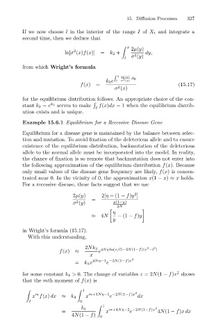
If we now choose l in the interior of the range I of X t and integrate a
second time, then we deduce that
x
2µ(y)
2
ln[σ (x)f(x)]
dy,
2
σ (y)
from which Wright’s formula = k 2 + l 15. Diffusion Processes 327
x 2µ(y)
"
dy
k 3 e l σ 2 (y)
f(x) = (15.17)
2
σ (x)
for the equilibrium distribution follows. An appropriate choice of the con-
"
stant k 3 = e k 2 serves to make f(x)dx = 1 when the equilibrium distrib-
I
ution exists and is unique.
Example 15.6.1 Equilibrium for a Recessive Disease Gene
Equilibrium for a disease gene is maintained by the balance between selec-
tion and mutation. To avoid fixation of the deleterious allele and to ensure
existence of the equilibrium distribution, backmutation of the deleterious
allele to the normal allele must be incorporated into the model. In reality,
the chance of fixation is so remote that backmutation does not enter into
the following approximation of the equilibrium distribution f(x). Because
only small values of the disease gene frequency are likely, f(x) is concen-
trated near 0. In the vicinity of 0, the approximation x(1 − x) ≈ x holds.
For a recessive disease, these facts suggest that we use
2
2µ(y) 2[η − (1 − f)y ]
=
2
σ (y) y(1−y)
2N

η
≈ 4N − (1 − f)y
y
in Wright’s formula (15.17).
With this understanding,
2
2
2Nk 3 4Nη ln(x/l)−2N(1−f)(x −l )
f(x) ≈ e
x
= k 4 x 4Nη−1 −2N(1−f)x 2
e
2
for some constant k 4 > 0. The change of variables z =2N(1 − f)x shows
that the mth moment of f(x)is
1
2
m
x f(x) dx ≈ k 4 x m+4Nη−1 −2N(1−f)x dx
e
I 0
1
k 4 m+4Nη−2 −2N(1−f)x 2
= x e 4N(1 − f)xdx
4N(1 − f) 0