Page 344 - Applied Probability

15. Diffusion Processes
333
it is useful to let
1
j −
2
=
a ij
2N i
for 0 ≤ j ≤ q and some positive integer q. The remaining a ij are distributed
over the interval [a iq , 1] less uniformly. This tactic separates the possibility
of exactly j alleles at time t i ,0 ≤ j ≤ q, from other possibilities. For
0 ≤ j ≤ q, binomial sampling dictates that

2N i+1 l 2N i+1 −l
p ij→i+1,k = p (1 − p)
l
l

1 2N i+1 l l 2N i+1 −l
= p (1 − p)
c ij→i+1,k
p ij→i+1,k l 2N i+1
l
where p = m(i, x) is the gamete pool probability at frequency x = j/(2N i)
and the sums occur over all l such that l/(2N i+1) ∈ [a i+1,k ,a i+1,k+1 ). When
0 ≤ k ≤ q, it is sensible to set c ij→i+1,k = k/(2N i+1 ).
density of X t

160
140
120
100
80
80
60
70
40 60
20 50
40
0 generations t
0 30
0.005
0.01 20
0.015
0.02 10
0.025
allele frequency X t 0.03
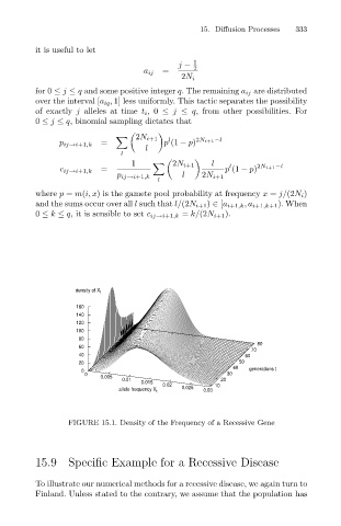
FIGURE 15.1. Density of the Frequency of a Recessive Gene

15.9 Specific Example for a Recessive Disease

To illustrate our numerical methods for a recessive disease, we again turn to
Finland. Unless stated to the contrary, we assume that the population has