Page 40 - Applied Probability

2. Counting Methods and the EM Algorithm
iteration m
2
p
mA
n m,A/A
people to genotype A/A and = n A p 2 mA +2p mAp mO 23
2p mAp mO
n m,A/O = n A 2
p +2p mAp mO
mA
people to genotype A/O. We now update p mA by
2n m,A/A + n m,A/O + n AB
p m+1,A = . (2.2)
2n
The update for p mB is the same as (2.2) except for the interchange of the
labels A and B. The update for p mO is equally intuitive and preserves
the counting requirement p mA + p mB + p mO = 1. This iterative proce-
dure continues until p mA, p mB , and p mO converge. Their converged values
p ∞A , p ∞B , and p ∞O provide allele frequency estimates. This gene-counting
algorithm [12] is a special case of the EM algorithm.

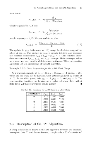
Example 2.2.2 Gene Frequencies for the ABO Blood Group
As a practical example, let n A = 186, n B = 38, n AB = 13, and n O = 284.
These are the types of 521 duodenal ulcer patients gathered by Clarke et
al. [2]. As an initial guess, take p 0A = .3, p 0B = .2, and p 0O = .5. The
gene-counting iterations can be done on a pocket calculator. It is evident
from Table 2.2 that convergence occurs quickly.

TABLE 2.2. Iterations for ABO Duodenal Ulcer Data
Iteration m p mA p mB p mO
0 .3000 .2000 .5000
1 .2321 .0550 .7129
2 .2160 .0503 .7337
3 .2139 .0502 .7359
4 .2136 .0501 .7363
5 .2136 .0501 .7363

2.3 Description of the EM Algorithm

A sharp distinction is drawn in the EM algorithm between the observed,
incomplete data Y and the unobserved, complete data X of a statistical