Page 42 - Applied Probability

2. Counting Methods and the EM Algorithm
25
2
(w−u)
is positive
If h(w) is strictly convex, then the neglected term h (v)

2
whenever w = u.
The next proposition uses the language of measure theory. To assist
readers unfamiliar with the subject, it is fair to point out that in practical
applications most measures reduce to ordinary length, area, or volume for
continuous random variables and to counting for discrete random variables.
In the former case, we integrate, and in the later case, we sum. The term
“almost everywhere” is the counterpart of “almost surely” in probability
theory and can be interpreted as everywhere with little harm.
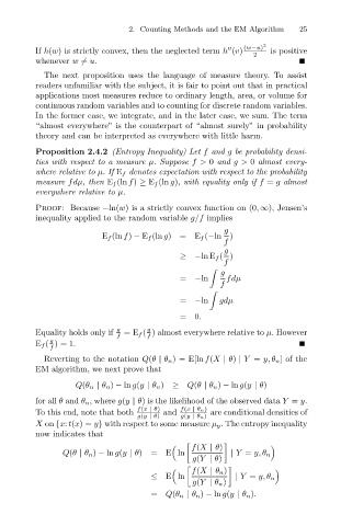
Proposition 2.4.2 (Entropy Inequality) Let f and g be probability densi-
ties with respect to a measure µ. Suppose f> 0 and g> 0 almost every-
where relative to µ.If E f denotes expectation with respect to the probability
measure fdµ, then E f (ln f) ≥ E f (ln g), with equality only if f = g almost
everywhere relative to µ.
Proof: Because −ln(w) is a strictly convex function on (0, ∞), Jensen’s
inequality applied to the random variable g/f implies
g
E f (ln f) − E f (ln g)=E f (−ln )
f
g
≥−ln E f ( )
f
g

= −ln fdµ
f

= −ln gdµ
=0.
g
Equality holds only if g =E f ( ) almost everywhere relative to µ. However
f f
g
E f ( )= 1.
f
Reverting to the notation Q(θ | θ n ) = E[ln f(X | θ) | Y = y, θ n ] of the
EM algorithm, we next prove that
Q(θ n | θ n ) − ln g(y | θ n ) ≥ Q(θ | θ n ) − ln g(y | θ)
for all θ and θ n , where g(y | θ) is the likelihood of the observed data Y = y.
f(x | θ) f(x | θ n )
To this end, note that both and are conditional densities of
g(y | θ) g(y | θ n )
X on {x: t(x)= y} with respect to some measure µ y . The entropy inequality
now indicates that

f(X | θ)

Q(θ | θ n ) − ln g(y | θ) = E ln | Y = y, θ n
g(Y | θ)

f(X | θ n )

≤ E ln | Y = y, θ n
g(Y | θ n )
= Q(θ n | θ n ) − ln g(y | θ n ).