Page 46 - Applied Probability

2. Counting Methods and the EM Algorithm
29
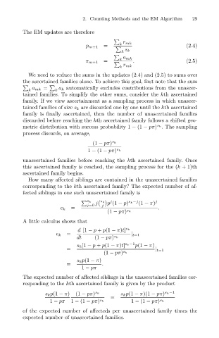
The EM updates are therefore
p m+1

s k

a mk
(2.5)
=
π m+1 = k k k r mk . (2.4)

r
k mk
We need to reduce the sums in the updates (2.4) and (2.5) to sums over
the ascertained families alone. To achieve this goal, first note that the sum

a mk = a k automatically excludes contributions from the unascer-
k k
tained families. To simplify the other sums, consider the kth ascertained
family. If we view ascertainment as a sampling process in which unascer-
tained families of size s k are discarded one by one until the kth ascertained
family is finally ascertained, then the number of unascertained families
discarded before reaching the kth ascertained family follows a shifted geo-
metric distribution with success probability 1 − (1 − pπ) . The sampling
s k
process discards, on average,
(1 − pπ) s k
s
1 − (1 − pπ) k
unascertained families before reaching the kth ascertained family. Once
this ascertained family is reached, the sampling process for the (k + 1)th
ascertained family begins.
How many affected siblings are contained in the unascertained families
corresponding to the kth ascertained family? The expected number of af-
fected siblings in one such unascertained family is

s k j s k p (1 − p) (1 − π)
j s k −j j
j=0 j
= .
e k s
(1 − pπ) k
A little calculus shows that
d [1 − p + p(1 − π)t] s k
=
e k s | t=1
dt (1 − pπ) k
s k [1 − p + p(1 − π)t] s k −1 p(1 − π)
= | t=1
s
(1 − pπ) k
s k p(1 − π)
= .
1 − pπ
The expected number of affected siblings in the unascertained families cor-
responding to the kth ascertained family is given by the product
s k p(1 − π) (1 − pπ) s k s k p(1 − π)(1 − pπ) s k −1
=
s
s
1 − pπ 1 − (1 − pπ) k 1 − (1 − pπ) k
of the expected number of affecteds per unascertained family times the
expected number of unascertained families.