Page 45 - Applied Probability

2. Counting Methods and the EM Algorithm
28
the investigator must correct for the ascertainment process. The simplest
ascertainment model postulates that the number of ascertained siblings fol-
lows a binomial distribution with success probability π and number of trials
equal to the number of affected siblings. In effect, families are ascertained
only through their affected siblings, and siblings come to the attention of
the genetic investigator independently, with common probability π per sib-
ling. The number of affecteds likewise follows a binomial distribution with
success probability p and number of trials equal to the number of siblings.
The EM algorithm can be employed to estimate p and π jointly. More
complicated and realistic ascertainment models are discussed in [14].
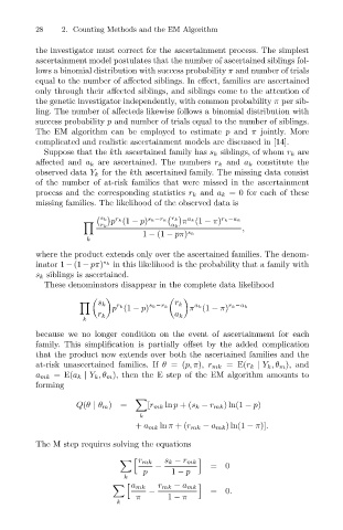
Suppose that the kth ascertained family has s k siblings, of whom r k are
affected and a k are ascertained. The numbers r k and a k constitute the
observed data Y k for the kth ascertained family. The missing data consist
of the number of at-risk families that were missed in the ascertainment
process and the corresponding statistics r k and a k = 0 for each of these
missing families. The likelihood of the observed data is

s k r k s k −r k r k a k r k −a k
p (1 − p) π (1 − π)
r k a k ,
s
1 − (1 − pπ) k
k
where the product extends only over the ascertained families. The denom-
inator 1 − (1 − pπ) s k in this likelihood is the probability that a family with
s k siblings is ascertained.
These denominators disappear in the complete data likelihood

s k r k

p (1 − p) s k −r k π (1 − π) r k −a k
a k
r k
r k a k
k
because we no longer condition on the event of ascertainment for each
family. This simplification is partially offset by the added complication
that the product now extends over both the ascertained families and the
at-risk unascertained families. If θ =(p, π), r mk =E(r k | Y k ,θ m ), and
a mk =E(a k | Y k ,θ m ), then the E step of the EM algorithm amounts to
forming

Q(θ | θ m ) = [r mk ln p +(s k − r mk )ln(1 − p)
k
+ a mk ln π +(r mk − a mk )ln(1 − π)].

The M step requires solving the equations

r mk s k − r mk
− =0
p 1 − p
k

a mk r mk − a mk
− =0.
π 1 − π
k