Page 49 - Applied Probability

2. Counting Methods and the EM Algorithm
32
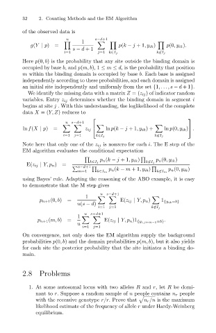
of the observed data is
u
s−d+1
1

p(k − j +1,y ik )
p(0,y ik ).
g(Y | p)=
s − d +1
i=1
k ∈I j
j=1 k∈I j
Here p(0,b) is the probability that any site outside the binding domain is
occupied by base b, and p(m, b), 1 ≤ m ≤ d, is the probability that position
m within the binding domain is occupied by base b. Each base is assigned
independently according to these probabilities, and each domain is assigned
an initial site independently and uniformly from the set {1,...,s − d +1}.
We identify the missing data with a matrix Z =(z ij ) of indicator random
variables. Entry z ij determines whether the binding domain in segment i
begins at site j . With this understanding, the loglikelihood of the complete
data X =(Y, Z) reduces to
 
u s−d+1

ln f(X | p)= z ij  ln p(k − j +1,y ik )+ ln p(0,y ik ) .

i=1 j=1 k∈I j k ∈I j
Note here that only one of the z ij is nonzero for each i. The E step of the
EM algorithm evaluates the conditional expectation

p n (k − j +1,y ik ) p n (0,y ik )
k∈I j k ∈I j
E(z ij | Y, p n )=
s−d+1 p n (k − m +1,y ik ) p n (0,y ik )
m=1 k∈I m k ∈I m
using Bayes’ rule. Adapting the reasoning of the ABO example, it is easy
to demonstrate that the M step gives
u s−d+1
1
p n+1 (0,b)= E(z ij | Y, p n ) 1 {y ik =b}
u(s − d)
i=1 j=1 k ∈I j
u s−d+1
1
p n+1 (m, b)= E(z ij | Y, p n)1 {y i,j+m−1 =b} .
u
i=1 j=1
On convergence, not only does the EM algorithm supply the background
probabilities p(0,b) and the domain probabilities p(m, b), but it also yields
for each site the posterior probability that the site initiates a binding do-
main.
2.8 Problems
1. At some autosomal locus with two alleles R and r,let R be domi-
nant to r. Suppose a random sample of n people contains n r people

with the recessive genotype r/r. Prove that n r /n is the maximum
likelihood estimate of the frequency of allele r under Hardy-Weinberg
equilibrium.