Page 59 - Applied Probability

3. Newton’s Method and Scoring
42
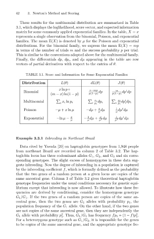
These results for the multinomial distribution are summarized in Table
3.1, which displays the loglikelihood, score vector, and expected information
matrix for some commonly applied exponential families. In the table, X = x
represents a single observation from the binomial, Poisson, and exponential
families. The mean E(X) is denoted by µ for the Poisson and exponential
distributions. For the binomial family, we express the mean E(X)= mp
in terms of the number of trials m and the success probability p per trial.
This is similar to the conventions adopted above for the multinomial family.
Finally, the differentials dp, dp i , and dµ appearing in the table are row
vectors of partial derivatives with respect to the entries of θ.
TABLE 3.1. Score and Information for Some Exponential Families
Distribution L(θ) dL(θ) J(θ)
x ln p+ x−mp
t
Binomial dp m dp dp
(m − x)ln(1 − p) p(1−p) p(1−p)
m t
Multinomial x i ln p i x i dp i dp dp i
i i p i i p i i
x
t
Poisson −µ + x ln µ −dµ + dµ 1 dµ dµ
µ µ
1
1
x
t
Exponential −ln µ − x − dµ + µ 2 dµ µ 2 dµ dµ
µ µ
Example 3.3.1 Inbreeding in Northeast Brazil
Data cited by Yasuda [20] on haptoglobin genotypes from 1,948 people
from northeast Brazil are recorded in column 2 of Table 3.2. The hap-
toglobin locus has three codominant alleles G 1 , G 2 , and G 3 and six corre-
sponding genotypes. The slight excess of homozygotes in these data sug-
gests inbreeding. Now the degree of inbreeding in a population is captured
by the inbreeding coefficient f, which is formally defined as the probability
that the two genes of a random person at a given locus are copies of the
same ancestral gene. Column 3 of Table 3.2 gives theoretical haptoglobin
genotype frequencies under the usual conditions necessary for genetic equi-
librium except that inbreeding is now allowed. To illustrate how these fre-
quencies are derived by conditioning, consider the homozygous genotype
G 1 /G 1 . If the two genes of a random person are copies of the same an-
cestral gene, then the two genes are G 1 alleles with probability p 1 , the
population frequency of the G 1 allele. On the other hand, if the two genes
are not copies of the same ancestral gene, then they are independently the
2
2
G 1 allele with probability p . Thus, G 1 /G 1 has frequency fp 1 +(1 − f)p .
1
1
For a heterozygous genotype such as G 1 /G 2 , it is impossible for the genes
to be copies of the same ancestral gene, and the appropriate genotype fre-