Page 60 - Applied Probability

3. Newton’s Method and Scoring
quency is (1 − f)2p 1p 2 .
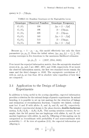
TABLE 3.2. Brazilian Genotypes at the Haptoglobin Locus
Genotype
2
fp 1 +(1 − f)p
108
G 1 /G 1 Observed Number Genotype Frequency 43
1
G 1 /G 2 196 (1 − f)2p 1p 2
429
G 1 /G 3 (1 − f)2p 1p 3
143 fp 2 +(1 − f)p 2
G 2 /G 2
2
513
G 2 /G 3 (1 − f)2p 2p 3
559 fp 3 +(1 − f)p 2
G 3 /G 3
3
Because p 3 =1 − p 1 − p 2 , this model effectively has only the three
1 1
parameters (p 1 ,p 2 ,f). From the initial values, (p 01 ,p 02 ,f 0 )=( , ,.02),
3 3
scoring converges in five iterations to the maximum likelihood estimates
ˆ
(ˆ p 1 , ˆ p 2 , f)=(.2157,.2554,.0431).
If we invert the expected information matrix, then the asymptotic standard
ˆ
errors of ˆ p 1 ,ˆ p 2 , and f are .0067, .0071, and .0166, respectively. If we invert
the observed information matrix, the first two standard errors remain the
same and the third changes to .0165. The asymptotic correlations of f ˆ
with ˆ p 1 and ˆ p 2 are less than .02 in absolute value regardless of how they
are computed.
3.4 Application to the Design of Linkage
Experiments

In addition to being useful in the scoring algorithm, expected information
provides a criterion for the rational design of genetic experiments. In animal
breeding, it is possible to set up test matings for the detection of linkage
and estimation of recombination fractions. Consider two linked, codomi-
nant loci A and B with alleles A 1 and A 2 and B 1 and B 2 , respectively.
The simplest experimental design is the phase-known, double-backcross
mating A 1 B 1 /A 2 B 2 × A 1 B 1 /A 1 B 1 . This mating notation conveys, for ex-
ample, that the left parent has one haplotype with alleles A 1 and B 1 and
another haplotype with alleles A 2 and B 2 . Offspring of this mating can be
categorized as recombinant with probability θ and nonrecombinant with
probability 1 − θ. In view of equation (3.5), the expected information per
offspring is
1 1
J(θ) = +
θ 1 − θ