Page 83 - Applied Probability

4. Hypothesis Testing and Categorical Data
66
With these definitions in mind, note first the obvious initial values (a)
t 0,k,1 = 1 for k< d, (b) t 0,k,1 = 0 for k ≥ d, and (c) t j,k,1 = 1 for j> 0.
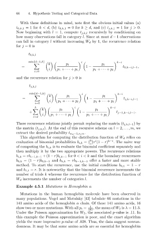
Now beginning with l = 1, compute t j,k,l recursively by conditioning on
how many observations fall in category l. Since at most d − 1 observations
can fall in category l without increasing W d by 1, the recurrence relation
for j =0 is
t 0,k,l
i k−i
min{d−1,k}
k p l p l
= 1 − t 0,k−i,l−1 ,
i p 1 + ··· + p l p 1 + ··· + p l
i=0
and the recurrence relation for j> 0is
t j,k,l
i k−i
min{d−1,k}
k p l p l
= 1 − t j,k−i,l−1
i p 1 + ··· + p l p 1 + ··· + p l
i=0
i
k k−i
k p l p l
+ 1 − t j−1,k−i,l−1 .
i p 1 + ··· + p l p 1 + ··· + p l
i=d
These recurrence relations jointly permit replacing the matrix (t j,k,l−1 )by
the matrix (t j,k,l ). At the end of this recursive scheme on l =2,... ,m,we
extract the desired probability t w d −1,n,m .
This algorithm for computing the distribution function of W d relies on
k
i k−i
evaluation of binomial probabilities b i,k = r (1 − r) . The naive way
i
of computing the b i,k is to evaluate the binomial coefficient separately and
then multiply it by the two appropriate powers. The recurrence relations
b i,k = rb i−1,k−1 +(1 − r)b i,k−1 for 0 <i <k and the boundary recurrences
b 0,k =(1 − r)b 0,k−1 and b k,k = rb k−1,k−1 offer a faster and more stable
method. To start the recurrence, use the initial conditions b 0,1 =1 − r
and b 1,1 = r. It is noteworthy that the binomial recurrence increments the
number of trials k whereas the recurrence for the distribution function of
W d increments the number of categories l.
Example 4.5.1 Mutations in Hemoglobin α

Mutations in the human hemoglobin molecule have been observed in
many populations. Vogel and Motulsky [43] tabulate 66 mutations in the
141 amino acids of the hemoglobin α chain. Of these 141 amino acids, 16
show two or more mutations. With all p i = 1 , the mean of W 2 is λ =11.3.
141
Under the Poisson approximation for W 2 , the associated p-value is .11. In
this example the Poisson approximation is poor, and the exact algorithm
yields the more impressive p-value of .028. Thus, the data suggest nonran-
domness. It may be that some amino acids are so essential for hemoglobin