Page 158 - Applied Statistics And Probability For Engineers

c04.qxd 5/10/02 5:20 PM Page 136 RK UL 6 RK UL 6:Desktop Folder:TEMP WORK:MONTGOMERY:REVISES UPLO D CH114 FIN L:Quark Files:

136 CHAPTER 4 CONTINUOUS RANDOM VARIABLES AND PROBABILITY DISTRIBUTIONS

1
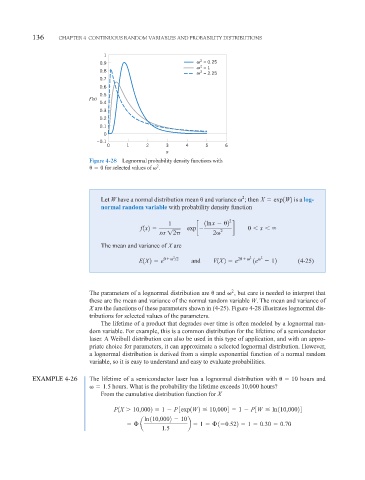
0.9 ω 2 = 0.25
ω 2 = 1
0.8 ω 2 = 2.25
0.7
0.6
0.5
f (x)
0.4
0.3
0.2
0.1
0
–0.1
0 1 2 3 4 5 6
x
Figure 4-28 Lognormal probability density functions with
0 for selected values of 2 .

Let W have a normal distribution mean and variance 2 ; then X exp1W2 is a log-
normal random variable with probability density function

2
1 1ln x 2
f 1x2 exp c d 0 x
x 12
2 2
The mean and variance of X are

2
E1X 2 e
2 and V1X 2 e 2
2 1e 2 12 (4-25)

The parameters of a lognormal distribution are and 2 , but care is needed to interpret that
these are the mean and variance of the normal random variable W. The mean and variance of
X are the functions of these parameters shown in (4-25). Figure 4-28 illustrates lognormal dis-
tributions for selected values of the parameters.
The lifetime of a product that degrades over time is often modeled by a lognormal ran-
dom variable. For example, this is a common distribution for the lifetime of a semiconductor
laser. A Weibull distribution can also be used in this type of application, and with an appro-
priate choice for parameters, it can approximate a selected lognormal distribution. However,
a lognormal distribution is derived from a simple exponential function of a normal random
variable, so it is easy to understand and easy to evaluate probabilities.

EXAMPLE 4-26 The lifetime of a semiconductor laser has a lognormal distribution with 10 hours and
1.5 hours. What is the probability the lifetime exceeds 10,000 hours?
From the cumulative distribution function for X

P1X 10,0002 1 P 3exp 1W 2 10,0004 1 P3W ln 110,00024
ln 110,0002 10
a b 1 1 0.522 1 0.30 0.70
1.5