Page 164 - Applied Statistics And Probability For Engineers

PQ220 6234F.CD(04) 5/13/02 11:55 M Page 2 RK UL 6 RK UL 6:Desktop Folder:TEMP WORK:MONTGOMERY:REVISES UPLO D CH114 FIN L:Quark

4-2 CHAPTER 4 CONTINUOUS RANDOM VARIABLES AND PROBABILITY DISTRIBUTIONS

A way to remember the approximation is to write the probability in terms of or and
then add or subtract the 0.5 correction factor to make the probability greater.
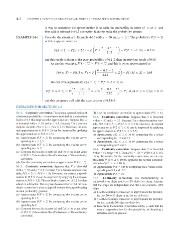
EXAMPLE S4-1 Consider the situation in Example 4-20 with n 50 and p 0.1 . The probability P1X 22
is better approximated as

2
0.5 5
P1X 22 P1X 2.52 P aZ b P1Z 1.182 0.119
2.12
and this result is closer to the exact probability of 0.112 than the previous result of 0.08.
As another example, P18 X2 P19 X2 and this is better approximated as
9 0.5 5
P19 X2 P18.5 X2 P a Zb P11.65 Z2 0.05
2.12

We can even approximate P1X 52 P15 X 52 as

5 0.5 5 5
0.5 5
P15 X 52 P a Z b P1 0.24 Z 0.242 0.19
2.12 2.12
and this compares well with the exact answer of 0.1849.

EXERCISES FOR SECTION 4-8
S4-1. Continuity correction. The normal approximation of (d) Use the continuity correction to approximate P(X
6).
a binomial probability is sometimes modified by a correction S4-3. Continuity correction. Suppose that X is binomial
factor of 0.5 that improves the approximation. Suppose that X with n 50 and p 0.1. Because X is a discrete random vari-
is binomial with n 50 and p 0.1 . Because X is a discrete able, P(2 X 5) P(1.5 X 5.5). However, the normal
random variable, P(X 2) P(X 2.5). However, the nor- approximation to P(2 X 5) can be improved by applying
mal approximation to P(X 2) can be improved by applying the approximation to P(1.5 X 5.5).
the approximation to P(X 2.5). (a) Approximate P(2 X 5) by computing the z-values
(a) Approximate P(X 2) by computing the z-value corre- corresponding to 1.5 and 5.5.
sponding to x 2.5. (b) Approximate P(2 X 5) by computing the z-values
(b) Approximate P(X 2) by computing the z-value corre- corresponding to 2 and 5.
sponding to x 2. S4-4. Continuity correction. Suppose that X is binomial
(c) Compare the results in parts (a) and (b) to the exact value with n 50 and p 0.1. Then, P(X 10) P(10 X 10).
of P(X 2) to evaluate the effectiveness of the continuity Using the results for the continuity corrections, we can ap-
correction. proximate P(10 X 10) by applying the normal standardi-
(d) Use the continuity correction to approximate P(X 10). zation to P(9.5 X 10.5).
S4-2. Continuity correction. Suppose that X is binomial (a) Approximate P(X 10) by computing the z-values corre-
with n 50 and p 0.1. Because X is a discrete random vari- sponding to 9.5 and 10.5.
able, P(X 2) P(X 1.5). However, the normal approxi- (b) Approximate P(X 5).
mation to P(X 2) can be improved by applying the approxi- S4-5. Continuity correction. The manufacturing of
mation to P(X 1.5). The continuity correction of 0.5 is either semiconductor chips produces 2% defective chips. Assume
added or subtracted. The easy rule to remember is that the con- that the chips are independent and that a lot contains 1000
tinuity correction is always applied to make the approximating chips.
normal probability greatest. (a) Use the continuity correction to approximate the probabil-
(a) Approximate P(X 2) by computing the z-value corre- ity that 20 to 30 chips in the lot are defective.
sponding to 1.5. (b) Use the continuity correction to approximate the probabil-
(b) Approximate P(X 2) by computing the z-value corre- ity that exactly 20 chips are defective.
sponding to 2. (c) Determine the number of defective chips, x, such that the
(c) Compare the results in parts (a) and (b) to the exact value normal approximation for the probability of obtaining x
of P(X 2) to evaluate the effectiveness of the continuity defective chips is greatest.
correction.