Page 168 - Applied Statistics And Probability For Engineers

c05.qxd 5/13/02 1:49 PM Page 144 RK UL 6 RK UL 6:Desktop Folder:TEMP WORK:MONTGOMERY:REVISES UPLO D CH114 FIN L:Quark Files:

144 CHAPTER 5 JOINT PROBABILITY DISTRIBUTIONS

and

f XY 12, 12 P1X 2, Y 12 0.0156

The probabilities for all points in Fig. 5-1 are shown next to the point and the figure describes
the joint probability distribution of X and Y.

5-1.2 Marginal Probability Distributions

If more than one random variable is defined in a random experiment, it is important to distin-
guish between the joint probability distribution of X and Y and the probability distribution of
each variable individually. The individual probability distribution of a random variable is re-
ferred to as its marginal probability distribution. In Example 5-1, we mentioned that the
marginal probability distribution of X is binomial with n 4 and p 0.9 and the marginal
probability distribution of Y is binomial with n 4 and p 0.08.
In general, the marginal probability distribution of X can be determined from the joint
probability distribution of X and other random variables. For example, to determine P(X x),
we sum P(X x, Y y) over all points in the range of (X, Y) for which X x. Subscripts on
the probability mass functions distinguish between the random variables.

EXAMPLE 5-3 The joint probability distribution of X and Y in Fig. 5-1 can be used to find the marginal prob-
ability distribution of X. For example,

P1X 32 P1X 3, Y 02 P1X 3, Y 12
0.0583 0.2333 0.292
As expected, this probability matches the result obtained from the binomial probability distribu-
1
3
4
tion for X; that is, P1X 32 1 3 20.9 0.1 0.292 . The marginal probability distribution for X
is found by summing the probabilities in each column, whereas the marginal probability distribu-
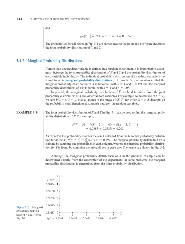
tion for Y is found by summing the probabilities in each row. The results are shown in Fig. 5-2.
Although the marginal probability distribution of X in the previous example can be
determined directly from the description of the experiment, in some problems the marginal
probability distribution is determined from the joint probability distribution.

y
(y) =
f Y
0.00004 4
0.00188 3
0.03250 2

0.24925 1
Figure 5-2 Marginal
probability distribu-
0.71637 0
tions of X and Y from 0 1 2 3 4 x
Fig. 5-1. f (x) = 0.0001 0.0036 0.0486 0.2916 0.6561
X