Page 172 - Applied Statistics And Probability For Engineers

c05.qxd 5/14/02 10:39 M Page 148 RK UL 6 RK UL 6:Desktop Folder:TEMP WORK:MONTGOMERY:REVISES UPLO D CH114 FIN L:Quark Files:

148 CHAPTER 5 JOINT PROBABILITY DISTRIBUTIONS

EXAMPLE 5-7 For the random variables in Example 5-1, the conditional mean of Y given X 2 is obtained
from the conditional distribution in Fig. 5-3:

E1Y 0 22 Y ƒ2 010.0402 110.3202 210.6402 1.6

The conditional mean is interpreted as the expected number of acceptable bits given that two
of the four bits transmitted are suspect. The conditional variance of Y given X 2 is
2
2
2
V1Y 0 22 10 Y ƒ2 2 10.0402 11 Y ƒ2 2 10.3202 12 Y ƒ2 2 10.6402 0.32
5-1.4 Independence

In some random experiments, knowledge of the values of X does not change any of the prob-
abilities associated with the values for Y.

EXAMPLE 5-8 In a plastic molding operation, each part is classified as to whether it conforms to color and
length specifications. Define the random variable X and Y as

1 if the part conforms to color specifications
X e
0 otherwise
1 if the part conforms to length specifications
Y e
0 otherwise

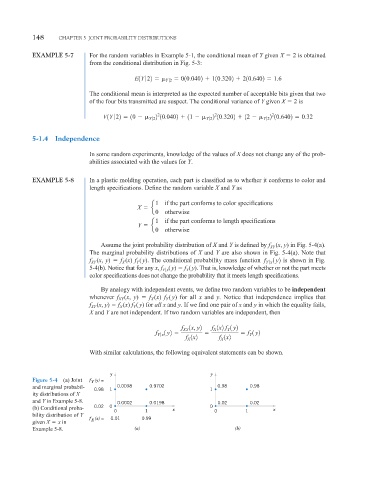
Assume the joint probability distribution of X and Y is defined by f (x, y) in Fig. 5-4(a).
XY
The marginal probability distributions of X and Y are also shown in Fig. 5-4(a). Note that
f (x, y) f (x) f (y). The conditional probability mass function f Y ƒ x 1 y2 is shown in Fig.
XY
X
Y
5-4(b). Notice that for any x, f (y) f (y). That is, knowledge of whether or not the part meets
Y x
Y
color specifications does not change the probability that it meets length specifications.
By analogy with independent events, we define two random variables to be independent
whenever f (x, y) f (x) f ( y) for all x and y. Notice that independence implies that
XY
X
Y
f (x, y) f (x) f (y) for all x and y. If we find one pair of x and y in which the equality fails,
XY
X
Y
X and Y are not independent. If two random variables are independent, then
f 1x, y2 f 1x2 f 1 y2
f Y ƒ x 1 y2 XY X Y f 1 y2
f 1x2 f 1x2 Y
X X
With similar calculations, the following equivalent statements can be shown.
y y
Figure 5-4 (a) Joint f (y) =
Y
and marginal probabil- 0.98 1 0.0098 0.9702 1 0.98 0.98
ity distributions of X
and Y in Example 5-8. 0.0002 0.0198 0.02 0.02
(b) Conditional proba- 0.02 0 0 1 x 0 0 1 x
bility distribution of Y
f X (x) = 0.01 0.99
given X x in
Example 5-8. (a) (b)