Page 182 - Applied Statistics And Probability For Engineers

c05.qxd 5/13/02 1:49 PM Page 158 RK UL 6 RK UL 6:Desktop Folder:TEMP WORK:MONTGOMERY:REVISES UPLO D CH114 FIN L:Quark Files:

158 CHAPTER 5 JOINT PROBABILITY DISTRIBUTIONS

f XY (x, y)

f XY (x, y)
y

R
y
x 7.80 x
3.05
Probability that (X, Y) is in the region R is determined 7.70 3.0
by the volume of f XY (x, y) over the region R. 7.60 2.95
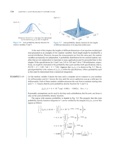
Figure 5-6 Joint probability density function for Figure 5-7 Joint probability density function for the lengths
random variables X and Y. of different dimensions of an injection-molded part.

At the start of this chapter, the lengths of different dimensions of an injection-molded part
were presented as an example of two random variables. Each length might be modeled by a
normal distribution. However, because the measurements are from the same part, the random
variables are typically not independent. A probability distribution for two normal random vari-
ables that are not independent is important in many applications and it is presented later in this
chapter. If the specifications for X and Y are 2.95 to 3.05 and 7.60 to 7.80 millimeters, respec-
tively, we might be interested in the probability that a part satisfies both specifications; that is,
P12.95 X 3.05, 7.60 Y 7.802. Suppose that f XY 1x, y2 is shown in Fig. 5-7. The re-
quired probability is the volume of f 1x, y2 within the specifications. Often a probability such
XY
as this must be determined from a numerical integration.
EXAMPLE 5-15 Let the random variable X denote the time until a computer server connects to your machine
(in milliseconds), and let Y denote the time until the server authorizes you as a valid user (in
milliseconds). Each of these random variables measures the wait from a common starting time
and X Y. Assume that the joint probability density function for X and Y is

f 1x, y2 6 10 6 exp1 0.001x 0.002y2 for x y
XY
Reasonable assumptions can be used to develop such a distribution, but for now, our focus is
only on the joint probability density function.
The region with nonzero probability is shaded in Fig. 5-8. The property that this joint
probability density function integrates to 1 can be verified by the integral of f XY (x, y) over this
region as follows:

f
° 6 10 e
XY 1x, y2 dy dx 6 0.001x 0.002y dy¢ dx

0 x

0.002y 0.001x
6
6 10 ° e dy¢ e dx
0 x

0.002x
e 0.001x
6
6 10 ° 0.002 ¢ e dx
0

0.003x 1
0.003 ° e dx¢ 0.003 a 0.003 b 1
0