Page 318 - Applied Statistics And Probability For Engineers

c08.qxd 5/15/02 6:13 PM Page 270 RK UL 6 RK UL 6:Desktop Folder:TEMP WORK:MONTGOMERY:REVISES UPLO D CH114 FIN L:Quark Files:

270 CHAPTER 8 STATISTICAL INTERVALS FOR A SINGLE SAMPLE

8-51. Consider the television tube brightness test described 8-56. How would you obtain a one-sided prediction bound
in Exercise 8-24. Compute a 99% prediction interval on the on a future observation? Apply this procedure to obtain a 95%
brightness of the next tube tested. Compare the length of the one-sided prediction bound on the wall thickness of the next
prediction interval with the length of the 99% CI on the popu- bottle for the situation described in Exercise 8-29.
lation mean. 8-57. Consider the fuel rod enrichment data described
8-52. Consider the margarine test described in Exercise 8-25. in Exercise 8-30. Compute a 99% prediction interval on the
Compute a 99% prediction interval on the polyunsaturated enrichment of the next rod tested. Compare the length of the
fatty acid in the next package of margarine that is tested. prediction interval with the length of the 95% CI on the
Compare the length of the prediction interval with the length population mean.
of the 99% CI on the population mean. 8-58. Consider the syrup dispensing measurements de-
8-53. Consider the test on the compressive strength of con- scribed in Exercise 8-31. Compute a 95% prediction interval
crete described in Exercise 8-26. Compute a 90% prediction on the syrup volume in the next beverage dispensed. Compare
interval on the next specimen of concrete tested. the length of the prediction interval with the length of the 95%
8-54. Consider the suspension rod diameter measurements CI on the population mean.
described in Exercise 8-27. Compute a 95% prediction inter- 8-59. Consider the natural frequency of beams described
val on the diameter of the next rod tested. Compare the length in Exercise 8-32. Compute a 90% prediction interval on the
of the prediction interval with the length of the 95% CI on the diameter of the natural frequency of the next beam of this
population mean. type that will be tested. Compare the length of the prediction
8-55. Consider the bottle wall thickness measurements interval with the length of the 95% CI on the population
described in Exercise 8-29. Compute a 90% prediction interval mean.
on the wall thickness of the next bottle tested.

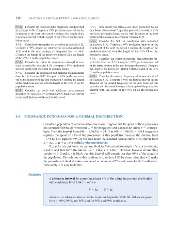
8-7 TOLERANCE INTERVALS FOR A NORMAL DISTRIBUTION

Consider a population of semiconductor processors. Suppose that the speed of these processors
has a normal distribution with mean 600 megahertz and standard deviation 30 mega-
hertz. Then the interval from 600 1.96(30) 541.2 to 600 1.96(30) 658.8 megahertz
captures the speed of 95% of the processors in this population because the interval from
1.96 to 1.96 captures 95% of the area under the standard normal curve. The interval from
z 2 to z 2 is called a tolerance interval.
If and are unknown, we can use the data from a random sample of size n to compute
x and s, and then form the interval 1x 1.96 s, x 1.96 s2 . However, because of sampling
x
variability in and s, it is likely that this interval will contain less than 95% of the values in
the population. The solution to this problem is to replace 1.96 by some value that will make
the proportion of the distribution contained in the interval 95% with some level of confidence.
Fortunately, it is easy to do this.

Definition
A tolerance interval for capturing at least % of the values in a normal distribution
with confidence level 100(1 )% is

x ks, x ks

where k is a tolerance interval factor found in Appendix Table XI. Values are given
for 90%, 95%, and 95% and for 95% and 99% confidence.