Page 342 - Applied Statistics And Probability For Engineers

c09.qxd 5/15/02 8:02 PM Page 290 RK UL 9 RK UL 9:Desktop Folder:

290 CHAPTER 9 TESTS OF HYPOTHESES FOR A SINGLE SAMPLE

N(0,1) N(0,1) N(0,1)
Critical region Critical region Critical region
α Acceptance α Acceptance α α Acceptance
/2
/2
region region region
–z α 0 z α Z 0 0 z α Z 0 –z α 0 Z 0
/2
/2
(a) (b) (c)
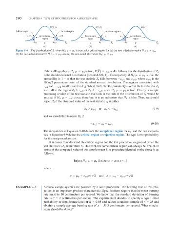
Figure 9-6 The distribution of Z 0 when H 0 : 0 is true, with critical region for (a) the two-sided alternative H 1 : 0 ,
(b) the one-sided alternative H 1 : 0 , and (c) the one-sided alternative H 1 : 0 .

If the null hypothesis H : is true, E1X 2 0 , and it follows that the distribution of Z 0
0
0
is the standard normal distribution [denoted N(0, 1)]. Consequently, if H : is true, the
0
0
probability is 1
that the test statistic Z falls between
z
2 and z
2 , where z
2 is the
0
100
2 percentage point of the standard normal distribution. The regions associated with
z
2 and
z
2 are illustrated in Fig. 9-6(a). Note that the probability is that the test statistic Z 0
will fall in the region Z z
2 or Z
z
2 when H : is true. Clearly, a sample
0
0
0
0
producing a value of the test statistic that falls in the tails of the distribution of Z would be
0
unusual if H : is true; therefore, it is an indication that H is false. Thus, we should
0
0
0
reject H if the observed value of the test statistic z is either
0
0
z z
2 or z
z
2 (9-9)
0
0
and we should fail to reject H if
0

z
2 z z
2 (9-10)
0
The inequalities in Equation 9-10 defines the acceptance region for H , and the two inequali-
0
ties in Equation 9-9 define the critical region or rejection region. The type I error probability
for this test procedure is .
It is easier to understand the critical region and the test procedure, in general, when the
test statistic is Z rather than . However, the same critical region can always be written in
X
0
x
terms of the computed value of the sample mean . A procedure identical to the above is as
follows:
Reject H : if either x a or x b
0
0
where
a z
2
1n and b
z
2
1n
0
0
EXAMPLE 9-2 Aircrew escape systems are powered by a solid propellant. The burning rate of this pro-
pellant is an important product characteristic. Specifications require that the mean burning
rate must be 50 centimeters per second. We know that the standard deviation of burning
rate is 2 centimeters per second. The experimenter decides to specify a type I error
probability or significance level of 0.05 and selects a random sample of n 25 and
obtains a sample average burning rate of x 51.3 centimeters per second. What conclu-
sions should be drawn?