Page 90 - Applied Statistics And Probability For Engineers

PQ220 6234F.Ch 03 13/04/2002 03:19 PM Page 68

68 CHAPTER 3 DISCRETE RANDOM VARIABLES AND PROBABILITY DISTRIBUTIONS

Now

E1X2 0f 102 1f 112 2f 122 3f 132 4f 142
010.65612 110.29162 210.04862 310.00362 410.00012
0.4

Although X never assumes the value 0.4, the weighted average of the possible values is 0.4.
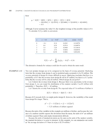
To calculate V1X2, a table is convenient.

x x 0.4 1x 0.42 2 f 1x2 f 1x21x 0.42 2
0 0.4 0.16 0.6561 0.104976
1 0.6 0.36 0.2916 0.104976
2 1.6 2.56 0.0486 0.124416
3 2.6 6.76 0.0036 0.024336
4 3.6 12.96 0.0001 0.001296

5
2
2
V1X2 a f 1x 21x 0.42 0.36
i
i
i 1
The alternative formula for variance could also be used to obtain the same result.
EXAMPLE 3-10 Two new product designs are to be compared on the basis of revenue potential. Marketing
feels that the revenue from design A can be predicted quite accurately to be $3 million. The
revenue potential of design B is more difficult to assess. Marketing concludes that there is a
probability of 0.3 that the revenue from design B will be $7 million, but there is a 0.7 proba-
bility that the revenue will be only $2 million. Which design do you prefer?
Let X denote the revenue from design A. Because there is no uncertainty in the revenue
from design A, we can model the distribution of the random variable X as $3 million with
probability 1. Therefore, E1X2 $3 million.
Let Y denote the revenue from design B. The expected value of Y in millions of dollars is

E1Y2 $710.32 $210.72 $3.5

Because E(Y) exceeds E(X), we might prefer design B. However, the variability of the result
from design B is larger. That is,

2 2 2
17 3.52 10.32 12 3.52 10.72
5.25 millions of dollars squared

Because the units of the variables in this example are millions of dollars, and because the vari-
ance of a random variable squares the deviations from the mean, the units of 2 are millions
of dollars squared. These units make interpretation difficult.
Because the units of standard deviation are the same as the units of the random variable,
the standard deviation is easier to interpret. In this example, we can summarize our results

as “the average deviation of Y from its mean is $2.29 million.’’