Page 215 - Applied statistics and probability for engineers

Section 5-6/Moment-Generating Functions 193

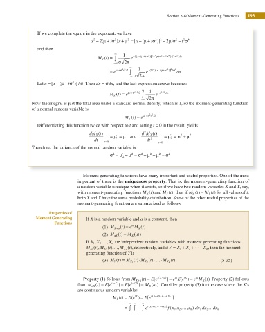
If we complete the square in the exponent, we have
x − 2(μ + tÈ 2 ) x +μ 2 = [ x − ( + È t 2 )] 2 −μ 2σ t 2 −σ t 2 4
μ
2
and then
∞
M t ( ) = ∫ 1 e − {[ x (− μ t + È 2 2 −2μ t σ 2 t − σ 2 4 } (2σ/ 2 ) dx
)]
X
−∞ σ 2π
∞ 1
2
2
= e μ t+È 2 2 ∫ e −( 1 2 x−( μ + σ )] / È 2 dx
)
t //2
/
[
t
−∞ σ 2π
Let u = [ x − (μ + tÈ 2 )] /σ . Then dx = σ du, and the last expression above becomes
∞ 1
M t) = e μ t+È 2 2 ∫ e −u 2 2 du
/
t /2
(
X
−∞ 2π
Now the integral is just the total area under a standard normal density, which is 1, so the moment-generating function
of a normal random variable is
M t) = e μ t+È 2 2 t /2
(
X
Differentiating this function twice with respect to t and setting t = 0 in the result, yields
2
dM t) = μ ’ = μ and d M t) = μ ′ = σ 2 + μ 2
(
(
X
X
dt 1 dt 2 2
t=0 t=0
Therefore, the variance of the normal random variable is
′
σ = μ 2 − μ = σ + μ − μ = σ 2
2
2
2
2
2
Moment generating functions have many important and useful properties. One of the most
important of these is the uniqueness property. That is, the moment-generating function of
a random variable is unique when it exists, so if we have two random variables X and Y, say,
with moment-generating functions M t( ) and M t( ), then if M t( ) = M t) for all values of t,
(
X
X
Y
Y
both X and Y have the same probability distribution. Some of the other useful properties of the
moment-generating function are summarized as follows.
Properties of
Moment Generating If X is a random variable and a is a constant, then
Functions
at
(1) M X a+ ( t = e M t)
(
)
X
(2) M aX ( = M at)
(
t)
X
If X X 2 , ,… X n are independent random variables with moment generating functions
1 ,
( ), t ( ), , t ( ), respectively, and if Y = X + X +⋯ + X n , then the moment
…
M X 1 t M X 2 M X n 1 2
generating function of Y is
(3) M t( ) = M X ( )⋅ 2 t)⋅ … ⋅ M X n t ( ) (5-35)
t M X (
Y
1
+
at
(
at
Property (1) follows from M X a+ ( t =) E e [ t X a) ] = e E e ( tX ) = e M t ( ). Property (2) follows
X
from M aX ( = E e [ t aX) ] = E e[ ( at X ] = M at). Consider property (3) for the case where the X’s
)
(
(
t)
X
are continuous random variables:
M t ( ) = E e ( tY ) = E e [ t X + 2 X n ) ]
X + +⋯
( 1
Y
∞ ∞ ∞
= ∫ ∫ ⋯ ∫ e t x ( + 2 x n ) f x x , , , x n ) dx dx z1 … dx n
x + +⋯
1
2 …
)
( 1
−∞ −∞ −∞