Page 318 - Applied statistics and probability for engineers

296 Chapter 8/Statistical intervals for a single sample

8-5 Guidelines for Constructing Confidence Intervals

The most dificult step in constructing a conidence interval is often the match of the appropri-
ate calculation to the objective of the study. Common cases are listed in Table 8-1 along with
the reference to the section that covers the appropriate calculation for a conidence interval
test. Table 8-1 provides a simple road map to help select the appropriate analysis. Two primary
comments can help identify the analysis:
1. Determine the parameter (and the distribution of the data) that will be bounded by the con-
idence interval or tested by the hypothesis.
2. Check if other parameters are known or need to be estimated.

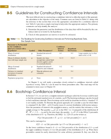
5"#-& t 8-1 The Roadmap for Constructing Confidence Intervals and Performing Hypothesis Tests,
One-Sample Case
Parameter to Be Bounded
by the Conidence Conidence
Interval or Tested with a Interval Hypothesis
Hypothesis? Symbol Other Parameters? Section Test Section Comments
Mean of normal μ Standard deviation σ 8-1 9-2 Large sample size is often
distribution known taken to be n ≥ 40
Mean of arbitrary distribu- μ Sample size large 8-1.5 9-2.5
tion with large sample size enough that central limit
theorem applies and σ
is essentially known
Mean of normal μ Standard deviation σ 8-2 9-3
distribution unknown and estimated
Variance (or standard σ 2 Mean μ unknown and 8-3 9-4
deviation) of normal estimated
distribution
Population proportion p None 8-4 9-5

In Chapter 9, we will study a procedure closely related to conidence intervals called
hypothesis testing. Table 8-1 can be used for those procedures also. This road map will be
extended to more cases in Chapter 10.
8.6 Bootstrap Confidence Interval

In Section 7-3.4, we saw how a computer-intensive technique called the bootstrap could be used
ˆ
to ind the estimated standard error of a statistic, say . θ The bootstrap technique can also be used
to ind conidence intervals. These bootstrap can be useful in situations in which a “standard” CI
is not readily available. To illustrate the general approach, let’s consider a case for which there
is a standard CI, the 100(1 – α)% CI on the mean of a normal distribution with known variance.
Here the parameter of interest is the population mean μ, and the statistic that estimates μ is the
sample average X. The quantity z α σ n is the 100( − ≠ 2) percentile of the distribution of
1
/2
θ i −
ˆ B θ B , i = 1 , ,… , n and by the same logic, the quantity −z α σ n is the 100(α 2) percentile
2
/2
B
(
of the distribution of X − μ. Therefore, the 100 1− α 2)% CI can be written as:
(
−
P α / 2th percentile ≤ X μ ≤ (1− α / )th percentile) = − α / 2
2
1
This can be rearranged as
(
α
P X − (1 − /2th ) percentile ≤ μ ≤ X + α /2th percentile ) = − /1 α 2
So the lower conidence bound is X − (1 α / )2 th percentile of the distribution of X − μ and
−
the upper conidence bound is X + α /2th percentile of the distribution of X − μ. When these
percentiles cannot be easily determined for some arbitrary parameter θ, they can often be