Page 320 - Applied statistics and probability for engineers

298 Chapter 8/Statistical intervals for a single sample

We noted in Section 8-2 that the t distribution based CI for μ was robust to the normal-
ity assumption when n is small. The practical implication of this is that although we have
computed a 95% CI, the actual coni dence level will not be exactly 95%, but it will be very
close—maybe 93% or 94%. Prediction intervals, on the other hand, are very sensitive to the
normality assumption, and Equaion 8-28 should not be used unless we are very comfortable
with the normality assumption.

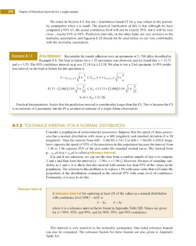
Example 8-11 Alloy Adhesion Reconsider the tensile adhesion tests on specimens of U-700 alloy described in
Example 8-6. The load at failure for n = 22 specimens was observed, and we found that x = 13.71
and s = 3.55. The 95% conidence interval on μ was 12 14 ≤ μ ≤ 15 28. We plan to test a 23rd specimen. A 95% predic-
.

.
tion interval on the load at failure for this specimen is
x − t / ,nα 2 −1 s 1 + 1 ≤ X n ≤ x + t / ,nα 2 −1 s 1 + 1
+1
n n
13 71−( 2 080 3 55 1+ 1 ≤ X 23 ≤ 13 71. +( 2 080 3 55 1 + 1
)
)
.
.
.
.
.
22 22
. ≤ 21 26
.
6 16 ≤ X 23
Practical Interpretation: Notice that the prediction interval is considerably longer than the CI. This is because the CI
is an estimate of a parameter, but the PI is an interval estimate of a single future observation.
8-7.2 TOLERANCE INTERVAL FOR A NORMAL DISTRIBUTION

Consider a population of semiconductor processors. Suppose that the speed of these proces-
sors has a normal distribution with mean μ = 600 megahertz and standard deviation σ = 30
megahertz. Then the interval from 600 – 1.96(30) = 541.2 to 600 + 1.96(30) = 658.8 mega-
hertz captures the speed of 95% of the processors in this population because the interval from
–1.96 to 1.96 captures 95% of the area under the standard normal curve. The interval from
μ − z α/2 È to μ + z È α/2 is called a tolerance interval.
If μ and σ are unknown, we can use the data from a random sample of size n to compute
(
x and s and then form the interval x − .1 96 s, x + .96 s). However, because of sampling vari-
1
ability in x and s, it is likely that this interval will contain less than 95% of the values in the
population. The solution to this problem is to replace 1.96 with some value that will make the
proportion of the distribution contained in the interval 95% with some level of coni dence.
Fortunately, it is easy to do this.

Tolerance Interval
A tolerance interval for capturing at least γ% of the values in a normal distribution

with conidence level 100(1 – α)% is
x − ks, x + ks
where k is a tolerance interval factor found in Appendix Table XII. Values are given
for γ = 90%, 95%, and 99%, and for 90%, 95%, and 99% coni dence.

This interval is very sensitive to the normality assumption. One-sided tolerance bounds
can also be computed. The tolerance factors for these bounds are also given in Appendix
Table XII.