Page 62 - Applied statistics and probability for engineers

40 Chapter 2/Probability

114 patients (67%), 82 of 112 patients (73%), 104 of 120 patients that the patient is in group 1, and let B denote the event that there is
(87%), and 113 of 121 patients (93%) in groups 1–4, respectively. no progression. Determine the following probabilities:
′
′
Suppose that a patient is selected randomly. Let A denote the event (a) P A( ∪ B) (b) P A( ′ ∪ B ) (c) P A( ∪ B )
2-4 Conditional Probability
Sometimes probabilities need to be reevaluated as additional information becomes available. A
useful way to incorporate additional information into a probability model is to assume that the out-
come that will be generated is a member of a given event. This event, say A, deines the conditions

that the outcome is known to satisfy. Then probabilities can be revised to include this knowledge.
The probability of an event B under the knowledge that the outcome will be in event A is denoted as
| (
P B A)
and this is called the conditional probability of B given A.
A digital communication channel has an error rate of 1 bit per every 1000 transmitted.
Errors are rare, but when they occur, they tend to occur in bursts that affect many consecutive
bits. If a single bit is transmitted, we might model the probability of an error as 1/1000. How-
ever, if the previous bit was in error because of the bursts, we might believe that the probability
that the next bit will be in error is greater than 1/1000.

In a thin ilm manufacturing process, the proportion of parts that are not acceptable is 2%.
However, the process is sensitive to contamination problems that can increase the rate of parts
that are not acceptable. If we knew that during a particular shift there were problems with the
ilters used to control contamination, we would assess the probability of a part being unac-

ceptable as higher than 2%.
In a manufacturing process, 10% of the parts contain visible surface laws and 25% of the parts

with surface laws are (functionally) defective parts. However, only 5% of parts without surface

laws are defective parts. The probability of a defective part depends on our knowledge of the pres-
ence or absence of a surface l aw. Let D denote the event that a part is defective, and let F denote

the event that a part has a surface law. Then we denote the probability of D given or assuming that
a part has a surface l aw, as P D F( | ). Because 25% of the parts with surface l aws are defective,
(
|
our conclusion can be stated as P D F) = .0 25. Furthermore, because F′ denotes the event that a

part does not have a surface law and because 5% of the parts without surface laws are defective,
(
0
|
we have P D F′) = .05. These results are shown graphically in Fig. 2-13.
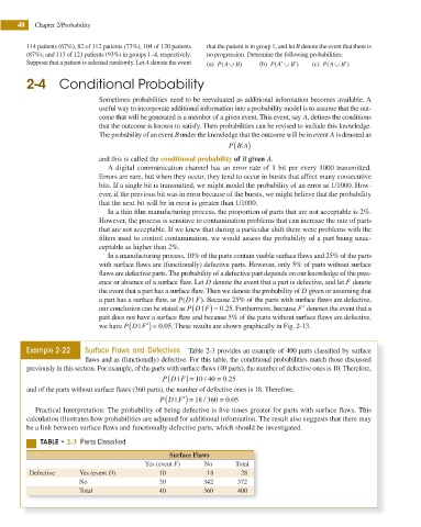
Example 2-22 Surface Flaws and Defectives Table 2-3 provides an example of 400 parts classii ed by surface

laws and as (functionally) defective. For this table, the conditional probabilities match those discussed
previously in this section. For example, of the parts with surface laws (40 parts), the number of defective ones is 10. Therefore,

(
|
0
/
P D F) = 10 40 = .25
and of the parts without surface laws (360 parts), the number of defective ones is 18. Therefore,

(
P D F′) = 18 360 = .05
/
0
|

Practical Interpretation: The probability of being defective is ive times greater for parts with surface l aws. This
calculation illustrates how probabilities are adjusted for additional information. The result also suggests that there may
be a link between surface laws and functionally defective parts, which should be investigated.

5"#-& t 2-3 Parts Classified
Surface Flaws
Yes (event F) No Total
Defective Yes (event D) 10 18 28
No 30 342 372
Total 40 360 400