Page 63 - Applied statistics and probability for engineers

Section 2-4/Conditional Probability 41

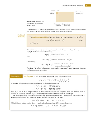
P(DuF) = 0.25
25% 5% defective
defective P(DuF') = 0.05

FIGURE 2-13 Conditional
probabilities for parts with F = parts with F' = parts without

surface flaws. surface flaws surface flaws
In Example 2-22, conditional probabilities were calculated directly. These probabilities can
also be determined from the formal deinition of conditional probability.

Conditional
Probability The conditional probability of an event B given an event A, denoted as P B A| ( ), is
P A∩ ) (
| (
P B A) = ( B / P A) (2-9)
for P A ( ) > 0.

This deinition can be understood in a special case in which all outcomes of a random experiment are
equally likely. If there are n total outcomes,
P A ( ) = (number of outcomes in A) / n
Also,
(
P A∩ B) = (number of outcomes in A ∩ B) / n
Consequently,
(
P A) =
P A∩ B) ( number of outcomes in A ∩ B
/
number of outcomes in A

| (
Therefore, P B A) can be interpreted as the relative frequency of event B among the trials that
produce an outcome in event A.
Example 2-23 Tree Diagram Again consider the 400 parts in Table 2-3. From this table,
(
P D F) = ( F P F) = 10 40 = 10
P D ∩ ) (
|
400 400 40
Note that in this example all four of the following probabilities are different:
/
( |
/
P F ( ) = 40 400 P F D) = 10 28
(
P D ( ) = 28 400/ P D F) = 10 40| /
(
Here, P D( ) and P D F| ) are probabilities of the same event, but they are computed under two different states of
(
knowledge. Similarly, P F( ) and P F D) are computed under two different states of knowledge.
|

The tree diagram in Fig. 2-14 can also be used to display conditional probabilities. The irst branch is on surface l aw. Of
the 40 parts with surface laws, 10 are functionally defective and 30 are not. Therefore,

(
(
|
/
P D F) = 10 40 and P D F) = 30 40′ | /

Of the 360 parts without surface laws, 18 are functionally defective and 342 are not. Therefore,
(
′ (
|
/
/
P D F′) = 18 360 and P D F′) = 342 360
|