Page 169 - Artificial Intelligence for the Internet of Everything

The Value of Information and the Internet of Things 155

The distribution of L is given by its density function f L (l). Modifying this
information changes the quantity we care about, that is:
What is the “value” of the information in items 5 and 6 of the previous list in how it
affects dhVie ? Does the shape of the graph change, does the maximum
b
behavior change, etc.?
We return to Eq. (9.4) to see the impact of changes in the information for
items 5 and 6. First, let us change the distribution of L so that it is uniformly
distributed on [0, L], L > 0, instead of [0, 2].
1
We see that PðL > bÞ¼ ðL bÞ, b L (0 for b > L). We see that, in
L
general, for and arbitrary positive μ we have:
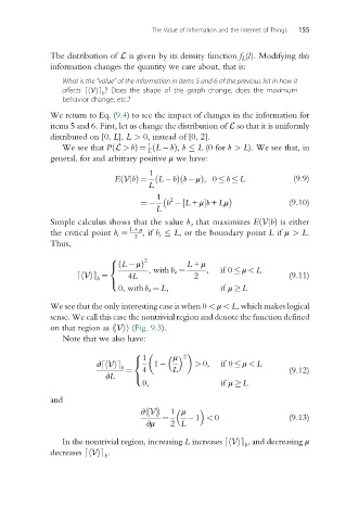
1
EðVjbÞ¼ ðL bÞðb μÞ,0 b L (9.9)
L

b ½L + μŠb + Lμ (9.10)
1 2
¼
L
Simple calculus shows that the value b o that maximizes EðVjbÞ is either
L + μ
the critical point b c ¼ 2 ,if b c L, or the boundary point L if μ > L.
Thus,
8 2 L + μ
ðL μÞ
, if 0 μ < L
<
4L 2 (9.11)
, with b o ¼
b
dhVie ¼
:
0, with b o ¼ L, if μ L
We see that the only interesting case is when 0 < μ < L, which makes logical
sense. We call this case the nontrivial region and denote the function defined
on that region as hhVii (Fig. 9.3).
Note that we also have:
μ

8 2
1
< > 0, if 0 μ < L
∂dhVie b 1
4 L (9.12)
∂L ¼ :
0, if μ L
and
1 μ

1 < 0 (9.13)
∂hhVii
∂μ ¼ 2 L
In the nontrivial region, increasing L increases dhVie , and decreasing μ
b
decreases dhVie .
b