Page 47 - Artificial Intelligence for the Internet of Everything

34 Artificial Intelligence for the Internet of Everything

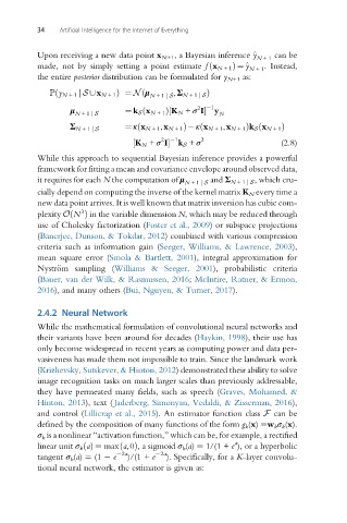
Upon receiving a new data point x N+1 , a Bayesian inference ^ N +1 can be
y
made, not by simply setting a point estimate f ðx N +1 Þ¼ ^y . Instead,
N +1
the entire posterior distribution can be formulated for y N+1 as:
ðy N +1 jS [x N +1 Þ¼ N ðμ
N +1 jS ,Σ N +1 jS Þ
2 1
μ ¼ k S ðx N +1 Þ½K N + σ IŠ y
N +1 jS N
¼ κðx N +1 ,x N +1 Þ κðx N +1 ,x N +1 Þk S ðx N +1 Þ
Σ N +1 jS
2 1
½K N + σ IŠ k S + σ 2 (2.8)
While this approach to sequential Bayesian inference provides a powerful
framework for fitting a mean and covariance envelope around observed data,
it requires for each N the computation of μ and Σ N +1 jS , which cru-
N +1 jS
cially depend on computing the inverse of the kernel matrix K N every time a
new data point arrives. It is well known that matrix inversion has cubic com-
3
plexity OðN Þ in the variable dimension N, which may be reduced through
use of Cholesky factorization (Foster et al., 2009) or subspace projections
(Banerjee, Dunson, & Tokdar, 2012) combined with various compression
criteria such as information gain (Seeger, Williams, & Lawrence, 2003),
mean square error (Smola & Bartlett, 2001), integral approximation for
Nystr€om sampling (Williams & Seeger, 2001), probabilistic criteria
(Bauer, van der Wilk, & Rasmussen, 2016; McIntire, Ratner, & Ermon,
2016), and many others (Bui, Nguyen, & Turner, 2017).

2.4.2 Neural Network
While the mathematical formulation of convolutional neural networks and
their variants have been around for decades (Haykin, 1998), their use has
only become widespread in recent years as computing power and data per-
vasiveness has made them not impossible to train. Since the landmark work
(Krizhevsky, Sutskever, & Hinton, 2012) demonstrated their ability to solve
image recognition tasks on much larger scales than previously addressable,
they have permeated many fields, such as speech (Graves, Mohamed, &
Hinton, 2013), text ( Jaderberg, Simonyan, Vedaldi, & Zisserman, 2016),
and control (Lillicrap et al., 2015). An estimator function class F can be
defined by the composition of many functions of the form g k (x) ¼w k σ k (x).
σ k is a nonlinear “activation function,” which can be, for example, a rectified
a
linear unit σ k ðaÞ¼ maxða,0Þ, a sigmoid σ k (a) ¼ 1/(1 + e ), or a hyperbolic
tangent σ k (a) ¼ (1 e 2a )/(1 + e 2a ). Specifically, for a K-layer convolu-
tional neural network, the estimator is given as: