Page 51 - Artificial Intelligence for the Internet of Everything

38 Artificial Intelligence for the Internet of Everything

2.5 ADVERSARIAL LEARNING IN DNN

Unfortunately these models have been shown to be very brittle and vulner-
able to specially crafted adversarial perturbations to examples: given an input
x and any target classification t, it is possible to find a new input x that is
0
similar to x but classified as t. These adversarial examples often appear almost
indistinguishable from natural data to human perception and are, as yet,
incorrectly classified by the neural network. Recent results have shown that
accuracy of neural networks can be reduced from close to 100% to below 5%
using adversarial examples. This creates a significant challenge in deploying
these deep learning models in security-critical domains where adversarial
activity is intrinsic, such as IoBT, cyber networks, and surveillance. The
use of neural networks in computer vision and speech recognition has
brought these models into the center of security-critical systems where
authentication depends on these machine-learned models. How do we
ensure that adversaries in these domains do not exploit the limitations of
ML models to go undetected or trigger an unintended outcome?
Multiple methods have been proposed in literature to generate adversar-
ial examples as well as defend against adversarial examples. Adversarial
example-generation methods include both white-box and black-box attacks
on neural networks (Goodfellow, Shlens, & Szegedy, 2014; Papernot et al.,
2017; Papernot, McDaniel, Jha, et al., 2016; Szegedy et al., 2013), targeting
feed-forward classification networks (Carlini & Wagner, 2016), generative
networks (Kos, Fischer, & Song, 2017), and recurrent neural networks
(Papernot, McDaniel, Swami, & Harang, 2016). These methods leverage
gradient-based optimization for normal examples to discover perturbations
that lead to misprediction—the techniques differ in defining the neighbor-
hood in which perturbation is permitted and the loss function used to guide
the search. For example, one of the earliest attacks (Goodfellow et al., 2014)
used a fast sign gradient method (FGMS) that looks for a similar image x in
0
∞
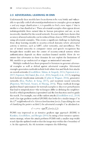
the L neighborhood of x. Given a loss function Loss(x, l) specifying the cost
of classifying the point x as label l, the adversarial example x is calculated as:
0
0
x ¼ x + E signðr x Lossðx,l x ÞÞ
FGMS was improved to an iterative gradient sign approach (IGSM) in
Kurakin, Goodfellow, and Bengio (2016) by using a finer iterative optimi-
zation strategy, where the attack performs FGMS with a smaller step-width
α and clips the updated result so that the image stays within the E boundary of
x. In this approach, the ith iteration computes the following: